METHOD AND RESULTS

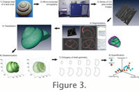As previously explained, the goal of this study is the development of a method allowing acquisition of quantitative morphometric parameters, which describe the geometry of coiled mollusc shells throughout their ontogeny. The approach proposed here includes the following major steps (Figure 3): 1) acquisition of digital three-dimensional data of the shell; 2) quantitative modelling of shell geometry; and 3) extraction of shell geometry through ontogeny.

Data acquisition by micro-computed tomography

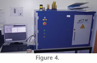In order to reconstruct the three-dimensional geometry of a gastropod shell, appropriate imaging techniques are required. A suitable and robust technique is the micro-computed tomography (micro-CT). This method is well known to allow non-destructive data acquisition of the external and internal geometry of anatomical structures with a high spatial resolution and a relatively fast acquisition time. It is commonly used in medical studies (Morton et al. 1990). In this study, the acquisition of digital three-dimensional data of gastropod shells is performed with a medical Scanco® micro-CT 80 (Figure 4) at the Anthropological Institute of Zürich.

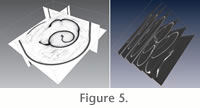The micro-CT produces a contiguous series of parallel two-dimensional images (Figure 5) obtained by scanning the original shell with X-rays (Ritman 2004). The pixels within each image slice are represented by scalar values that can be interpreted as intensity values (transparency to X-rays). Putting pixels and slices together we obtain a three-dimensional partition of the image space into volume elements (voxels) forming a 3-D scalar field. Regions of homogeneous intensity values typically represent anatomical structures, whereas strong gradients are indicators of tissue boundaries. Anatomical structures of interest can now be traced between adjacent images. Stacking those sliced structures on top of each other reveals an approximation of their three-dimensional shape.

In this study, gastropod shells are scanned with an isotropic voxel resolution of 0.036 mm. Usually, for a gastropod shell with a diameter of about 2 cm, the scanning process takes roughly 3 hours and results in a file size of about 2 Gb with a standard resolution of 1024 × 1024 pixels. The final size of a gastropod shell can be coded by a 3-D matrix of about 800 × 700 × 600 voxels. A full scan then yields a 3-D scalar field of about 4 × 10⁸ voxels. Medical images are typically stored in DICOM format.

Reconstruction of shell geometry

The next step is to reconstruct a three-dimensional, numerically exact descriptive model of the scanned shell. For this purpose, the series of images resulting from the micro-CT scan of a shell is transferred into a computer visualisation system. In this study, we use the commercial software amira®, which is a convenient and interactive system for 3-D data analysis, visualization and geometry reconstruction (Stalling et al. 2005). Algorithms used by amira® for image data analysis and geometry reconstruction are given by Zachow et al. (2007). The 3-D scalar fields resulting from the micro-CT scan of a shell can be visualized, and its structures can be analyzed in many different ways. We propose the following approach.

Many subsequent image analyses require data sets to be stored completely in random access memory (RAM) of the computer. Hence, raw data must fit the available RAM of the computer used for the shell 3-D reconstruction. For this purpose, the series of stacked images is first cropped to remove uninformative parts of the data set. If the data set is still too large with respect to the computer memory, it should be then down sampled.

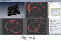
Raw scanned images may contain additional objects other than the shell (e.g., material to immobilize the shell during scanning, or remaining soft-tissues, or microscopic sand grains), as well as some "noisy" background values (Figure 5). The next step of the method is thus the segmentation of the stacked images. Segmentation is the process of dividing an image data into different segments for 3-D reconstruction, i.e., the process of selecting/identifying voxels belonging only to the shell in our case. The segmentation result is represented in the form of a 3-D label field. From micro-CT, each pixel in an image has a grey-scaled value, which corresponds to the relative density of the material at this spatial position. In our case, the segmentation process is rather simple since shells of living gastropods have a very high density compared to the surrounding air, which leads to highly contrasted images. 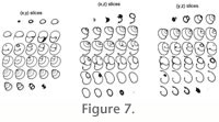Raw stacked images are thus threshold-segmented (Figure 6); see Sahoo et al. 1988 for an overview of various thresholding techniques. The result of this segmentation process is a series of 2-D binary images (Figure 7), i.e., black (0) and white (1). Computer memory considerations lead us to perform this step very early in the process. Indeed, segmentation significantly reduces data size by changing data type from signed integer (-32768→32767: 16 bits) to unsigned short integer (0→255: 8 bits).This reduction of size is important because it enables the analysis of larger, better resolved data sets.

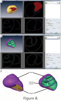It is noteworthy that most gastropods have a large overlap between successive whorls. The consequence is that it is impossible to reconstruct the shell geometry of covered parts of the shell from the external surface of the shell. To overcome this problem, we do not extract the shell itself, but its internal volume (i.e., the internal mould). Note that the internal surface of gastropod shells is usually smoothed compared to its external surface. To extract this internal volume, the shell is numerically bounded at its last aperture. Note that the shell is previously rotated so that the final shell aperture is contained in a plane parallel to the plane Oxy of the data set. This step is required by the software we used and may be unnecessary with another one. Note also that the real adult margin of the shell aperture is not planar. In order to have a closed outline, the shell aperture is actually bounded at its mature constriction, which is the nearest and most easily identifiable closed outline of the shell aperture (Figure 8.1). The internal volume of the shell is then easily identifiable by being bracketed between the shell itself and this stopper (Figure 8.2). Finally, the studied gastropod shell is segmented into the following parts (Figure 8.3): the shell itself, a stopper in the plane of the mature constriction, and the internal volume of the shell.

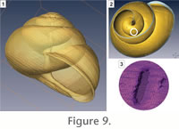
The shell may not be thick enough, especially in the innermost whorls, to be accurately detected by the tomograph nor selected during the segmentation process. This may create or artificially enlarge holes in the shell (Figure 9). Such holes complicate the subsequent geometric analyses by connecting successive whorls. Hence, the next step of the method is to apply a dilation operation of two voxels to the stacked images. This dilation enables the removal of (or at least reduce) most of these holes without changing the geometry of the shell.

At this step, the gastropod shell is represented by a 3-D matrix of integer values indicating to which segment each voxel belongs to. This voxel grid will be used later for extraction of a curve-skeleton (see below).

In the current state of data, the different segments of the gastropod shell (i.e., the shell itself, the stopper at the mature constriction, and the internal volume of the shell) can now be accurately reconstructed by tessellating their boundary surfaces from the 3-D image data. Tessellation consists in representing the segmented structure by a rather large set of piecewise linear surface primitives (triangles) that are convenient to render since graphics hardware is optimized for this goal. The internal volume of the gastropod shell is thus described by a triangular mesh, which basically is a connected array of three-dimensional triangles placed at its surface (Figure 10.1). Since the initial triangulation that is constructed from a segmented data volume occurs on sub-voxel resolution, the number of triangles might amount to several millions very quickly. 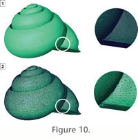The surface reconstruction is over-sampled, and a major requirement is the reduction of the high resolution via surface simplification (Figure 10.2). After this step, the user must test that the surface is closed and that the triangles are still consistently oriented and without intersections. Finally, for the following geometric analyses, the 3-D reconstruction (triangular mesh) of the internal volume of the shell is stored in a text file, which lists the three-dimensional coordinates of all vertices of the mesh and the three vertices of each triangle of the mesh.

Ontogenetic extraction of shell geometry

The last part of the method is the extraction of the shell geometry throughout ontogeny. In this study, we propose to recover the ontogenetic changes of the shell geometry by reconstructing and using a curve-skeleton. A curve-skeleton (or centreline, or medial axis, or central path) is a compact 1-D representation of 3-D objects, which is conceptually defined as the locus of centre voxels in the object. In this study, the curve-skeleton is expected to be placed at the centre of the shell aperture at each increment of growth. Due to its compact shape representation, skeletonization has been studied for a long time in pattern recognition (e.g., Trahanias 1992; Baseski et al. 2009), in medicine (e.g., quantification of anatomical structures or virtual navigation for colonoscopy: Pizer et al. 1999; Sorantin et al. 2002; Perchet et al. 2004) and in computer graphics (e.g., body animation or morphing: Blanding et al. 2000; Wade and Parent 2002).

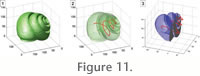
Although straightforward in 2-D, the extraction of a curve-skeleton in 3-D remains a difficult task. There exists a large number of methods, based on different kind of data (cloud points, polygonal mesh, or voxel grid); each one with advantages and drawbacks. For a review of major methods see Kirbas and Quek (2004) or Cornea et al. (2007). Briefly, the choice of the method is guided by the following aspects: preservation of the original object's topology and connectivity, centeredness of the curve, its thickness (one voxel width), its branching, its computing time and its noise sensitivity. In this study, we selected the potential field method (Chuang et al. 2000; Cornea et al. 2005), which can produce directly a smooth and single-branched skeleton. Briefly, the potential field method is basically a distance transform. It means that for each voxel of the shell, we calculate the Euclidean distance between this voxel and the nearest boundary voxel (i.e., a voxel placed on the surface of the shell). The raw skeleton is then derived by identifying the "sinks" of the distance field (i.e., the locally maximal distances), which are locally centred within the object, and by connecting them using a force following algorithm (see Cornea et al. 2005). In the potential field method, instead of using the shortest distance to the region border, a scalar function (the potential) is used (see Ahuja and Chuang 1997; Chuang et al. 2000). Practically the result of the extraction of a curve-skeleton is a series of 3-D points (Figure 11), which are extracted from the voxel grid.

The curve-skeleton of a gastropod shell is a very useful tool. It can be compared with the aperture trajectory (Stone 1995), although defined and calculated in a different way. It can be used as a guide to extract the geometry of a succession of whorl sections in an automated navigation throughout ontogeny of the shell. 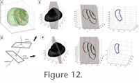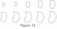The same idea is widely applied in medicine such as in virtual colonoscopy (e.g., Deschamps and Cohen 2001; Chaudhuri et al. 2004). For this purpose, successive cross-sections, centred on and perpendicular to the curve-skeleton, are computed along the curve-skeleton (Figure 12), by calculating the intersection of the corresponding cutting plane with the triangular mesh (Figure 12). The result is an ontogenetic series of successive outlines representing shell geometry (Figure 13). Note that this approach assumes that the shell aperture is within a 2-D plane, which is actually not the case. Even if the resolution of the micro-CT is enough to distinguish the growth lines, the whorl overlap of the shell prevents their use throughout ontogeny. Nevertheless, this 2-D approximation of the shell aperture remains sufficient to capture morphometric changes of the shell through ontogeny.

We now have a 3-D reconstruction of the gastropod shell throughout its ontogeny. The geometry of the shell can then be quantified by two sets of parameters. The first set is the displacement vector between two successive cross-sectioning planes. This vector records the translation and rotation coefficients between the origins of two successive cross-sectioning planes. The second set is the successive outlines of whorl sections through ontogeny. Since the whorl shape of gastropods may not have a sufficient number of landmarks to capture the shape (see Johnston et al. 1991), these data can be analyzed by outline analysis instead of landmark-based methods (see Adams et al. 2004). Three major approaches exist: eigenshape analysis (Lohmann 1983), elliptic Fourier analysis (Ferson et al. 1985) and the more recent sliding semi-landmark approach (Bookstein 1997; MacLeod 1999). Each outline is here quantified by elliptic Fourier analysis (EFA). This method is well suited to quantitatively model the complex outline of a shape in two or three spatial dimensions (Lestrel 1997; Haines and Crampton 1998; McLellan and Endler 1998). In general terms, Fourier analysis can be thought of as supplying the coefficients of a trigonometric function that reproduces as closely as possible a sample curve. As more terms (harmonics) are added to the function, the fit to the sample curve (in our case the aperture outline) becomes better. In EFA, the outline is characterized by a series of four coefficients for each selected harmonics. The number of harmonics necessary to reconstruct an outline depends on the complexity of this outline but usually does not exceed 20. The series of coefficients of the selected harmonics are then used as a mathematical characterization of the geometry of whorl sections.

The calculated coefficients of harmonics of a whorl section of the gastropod shell, coupled with the displacement vector (translation and rotation) between two successive cross-sectioning planes, constitute an n-dimensional morphometric space. The successive values of these harmonics and of the displacement vector of a single gastropod shell through ontogeny constitute a morphometric ontogenetic trajectory in this n-D space. The ontogenetic trajectories of each specimen and species can thus be analysed and compared quantitatively within this n-D space. The geometry of a shell is thus quantified by a set of multivariate data. The analysis of such data sets is standard in morphometrics, and one can find methodological developments and examples in Bookstein (1991), Marcus et al. (1996) and Zelditch et al. (2004), among others.