|
|
|
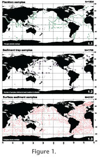
SOURCES AND METHODSSources of informationThis atlas is based on practically all the information available on the distribution of Recent polycystine radiolarians in the World Ocean. Information has been compiled from 91 different sources, including publications, Master and Doctoral dissertations, publicly available internet databases (PANGAEA, JGOFS), and unpublished records (Figure 1, Appendix 1). Our main target was reports that (1) covered at least a large majority of the radiolarian species in the samples (as opposed to papers dealing with one or a few selected species only), (2) included at least relative (%) abundance data, and (3) supplied basic station data unequivocally (mainly position and water depth). Nevertheless, we also covered several papers that provide binary (presence-absence) radiolarian data, works that dealt with only one or a few radiolarian species, as well as a few publications restricted to the assessment of radiolarian absolute abundances (i.e., cells per liter of water filtered - plankton samples, cells per square meter per day - sediment trap samples, and skeletons per g dry sediment - surface sediment samples). Appendix 1 provides an overview of the sources used and the type of information extracted from each. The database thus compiled covered the following information: • Source publication • Type of radiolarian data (presence-absence, species percentages, absolute density estimates, etc.) • Sample type (plankton, sediment trap, surface sediments) and identification • Sampler type • Type and depth of tow, volume of water filtered, net mesh size, date (for plankton samples) • Depth of trap, type of trap, dates of trap deployment (for sediment trap samples) • Sample preparation and analysis: sieve mesh size, number of radiolarians counted per sample • Latitude and longitude, bottom depth • Number of radiolarians per cubic meter of water fitered (plankton), per g of dry sediment (sediments), or per square meter per day (sediment traps) (when available). In some cases, the total numbers of samples included in our database (Appendix 1) may differ from the numbers reported by the corresponding author because we eliminated samples barren of polycystines (occasionally included in the original sample lists). On the other hand, samples with no polycystines in surveys aimed at absolute radiolarian abundances only were retained in our data.
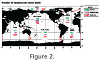
The North Pacific Ocean is by far better covered than any other area, both in absolute terms of number of samples and in terms of samples per unit surface. It is followed by the North Atlantic, with other oceanic areas lagging behind (Figure 2). When information was extracted from two or more partially overlapping sources the records in question were cross-checked in order to avoid duplicates. However, in a few cases, when the provenance of the data was not fully detailed in the source(s) duplicate information may have been retained in our database. We estimate that these duplicates represent <1% of the datapoints compiled.
Standarization of the data
Recent polycystines include a number of more or less well-established species whose characteristics are generally agreed upon and whose nomenclature is fairly stable among authors, and forms whose nomenclature is less uniform but whose restricted variability and rather well-defined morphology allows establishing synonyms easily and securely. Another category comprises problematic forms whose nomenclature varies widely among authors. In some cases these discrepancies can be traced to turn of the century monographs where several of Ehrenberg´s and Haeckel´s species were redescribed under new names. In most cases, however, morphological species concepts are more uniform and stable than species names, which allow grouping them under a single name with reasonable confidence. Species of these two categories were included in the database under the name currently most widely used. Synonyms were assigned on the basis of descriptions, illustrations, and/or synonyms provided by the author. In addition, when combining names, we considered the distributions of the taxa, so that if two similar forms had clearly different distribution ranges they were left separated. At the other end are the highly problematic forms, with very complicated and variable morphology, still requiring research to establish the species limits. In these cases we resorted to using less precise taxonomic categories such as "species groups". In extreme cases these forms were lumped under the corresponding family epithets. Summarizing, the names used by the original authors were maintained unless: 1. From the illustrations, descriptions, and/or synonymies provided it was clear that the same species had been reported under a different name by other authors. 2. The species is a member of a problematic group and is normally identified conditionally or in nomenclatura aperta (ex gr., aff., sp. or spp., s.l., etc.). In these cases we placed it either in an unresolved species group or under the corresponding family name. 3. The taxon consists of two or more very closely related morphotypes that were considered separately by one or a few authors, but were counted jointly by most others. In most of these cases the two forms were lumped in our review (e.g., Lamprocyclas maritalis maritalis, Lamprocyclas maritalis polypora and Lamprocyclas maritalis ventricosa; Didymocyrtis tetrathalamus tetrathalamus and Didymocyrtis tetrathalamus coronatus; etc.). In a few cases, especially when there was evidence that the siblings have dissimilar distributional ranges, we retained the three alternatives: records of sibling A, records of sibling B, and records of both siblings undifferentiated. 4. Some species that are newly erected, but inadequately described and illustrated. These were placed under the corresponding family level group. As a rule of thumb, species named differently in the original sources were merged only when there was clear evidence that we were dealing with synonyms. Whenever there were doubts about the status of a species, or evidence for merging it was considered inconclusive, the taxon was either left separated under the original name, or lumped in the corresponding "species group" or family (Appendix 2). Overall, our resulting database retained a very large proportion of the species treated in the original reports used for the compilation: on average, over 95% of the taxa with firm (i.e., non-conditional) identifications were incorporated into our database. Eleven of the species listed (Appendix 2) have no records in the database. This is because they have been figured and described (and are clearly valid species), but they have no records in the data compiled (ommitted in the counts by the corresponding author). These taxa are: Arachnosphaera sp. 1, Clathrocyclas sp. 1, Clathromitra pterophormis, Cromyomma sp. 1, Dictyophimus sp. 1, Heliosoma sp. 1, Liriospyris sp. 1, Phrenocodon clathrostomium, Plegmosphaera oblonga, Styptosphaera sp. 2, and Tetraplecta corynephorum?
Maps and graphsIllustrations depicting the quantitative distribution of radiolarian species are based on percentage data (either reported as such in the original paper, or recalculated from absolute or relative counting figures), and because of the nature of the information used, they are subject to some constraints: These representations assume that the totals of the samples involved include unidentified specimens so that the percentages in question are effectively of the overall assemblage, rather than proportions of identified specimens only. Data sets that did not meet this condition (e.g., Hays 1965), or recorded only binary information (presence-absence; e.g., Johnson and Nigrini 1980, 1982) were incorporated but with a notation that the taxon in question was present only. Percentage values are given only in those cases when the corresponding estimate was based on counts of a reasonably high number of specimens per sample. In some of the surveys used, the numbers of radiolarians per sample retrieved were extremely low, yielding unreliable percentage values. For the maps, we used a cutoff value of 50 identified specimens per sample; below this figure, the species (if recorded) is designated as "present" only. One of the problems of representating these data is associated with the absences of species. Negative records in original sources may result from different circumstances: (1) the species was looked for but was not found, or (2) the species was present in the sample(s) but was excluded from the counting categories used by the author. These two circumstances have quite different implications, yet their graphic representation is identical. We therefore indicated absences only for those data sets where the taxon was recorded at least once. Thus, its presence in at least one sample indicates that it has been searched for and recognized when present. For example: in the database of Hollis and Neil (2005) Didymocyrtis tetrathalamus was recorded in 11 of the 31 samples, therefore for the 20 samples where it was not found, it is denoted as absent in the maps. On the other hand, Casey (1971) did not include Didymocyrtis tetrathalamus (=Panartus tetrathalamus, =Ommatartus tetrathalamus) in his survey (although given its known distribution it must have been present in most of his samples, see below). Thus, in Casey´s (1971) mapped samples Didymocyrtis tetrathalamus is not indicated as absent. Because of the extremely high numbers of data points, and the fact that many of them overlap (especially in water-column materials), graphic representation of all the records on a reasonably sized map is impossible. Furthermore, because of the large sample-to-sample variability, it is more important in this type of review to offer a clear picture of the overall distributional trend, rather than to show all the raw, unprocessed information. Thus, in order to circumvent the problem of overlapping data points and extract meaningful trends from the data, distributional maps are based on information averaged for 5 x 5 degree Marsden squares. Graphic representation of summarized vertical distribution data is complicated by the fact that plankton tow intervals vary widely between surveys and are often not based on established oceanographic depth zones. To circumvent this problem for each plankton tow we calculated the central depth and subsequently used this value for grouping the vertical plankton data illustrated in the diagrams. In most cases the nominal (figured) depth interval is reasonably close to the actual depth interval sampled. In some, however, the intervals sampled were very large, in which case the nominal depth interval may not adequately reflect the actual depth interval sampled (see below).
List of species (Appendix 2)Taxa are listed alphabetically. For each entry the following information is given: species name, authority, family (in parentheses), up to 3 references illlustrating the species concept used ("Ref."), other names used variously for this species in the literature surveyed ("Other names"), and remarks ("Rem."). |
|
|
|