NUMBERS OF RADIOLARIAN SHELLS
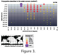 Vertical distribution of cell numbers (Figure 3) Vertical distribution of cell numbers (Figure 3)
Included are all plankton samples with absolute quantitative polycystine data. Depth intervals shown are calculated as half of the distance between the bottom and the top of each plankton tow. For example, for a tow from 550 to 320 m the mid-depth is 435 m [((550-320)/2)+320], and the corresponding data are included in the 300 to 500 nominal depth interval. Agreement between nominal and actual depth intervals is best in the upper 100 m where the mean difference between nominal and actual top and bottom depths is around 3 m.
 Between 100 and 500 m this mean difference is ca. 19 m, whereas at 500 to 5000 m it is around 90 m. Between 100 and 500 m this mean difference is ca. 19 m, whereas at 500 to 5000 m it is around 90 m.
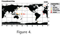
Polycystine fluxes (Figure 4)
Data illustrated are mean annual values based on sediment trap deployments of at least 9 consecutive months. Total sediment trap samples used for deriving the means: 905, total datapoints illustrated: 45.
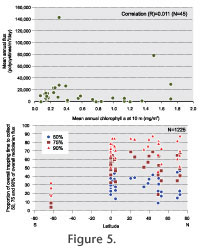 Polycystine fluxes vs. mean annual chlorophyll a and (Figure 5.1) Polycystine fluxes vs. mean annual chlorophyll a and (Figure 5.1)
Polycystine flux data are the same as those in
Figure 4. Chlorophyll data are mean annual values at 10 m depth (from
Conkright et al. 1998a,
1998b,
1998c).
Polycystine production half-time as a function of latitude (Figure 5.2)
Graph illustrates the time (as a percentage of overall trapping time) it takes to generate ?50, 75, and 90% of the overall radiolarian flux during the entire trapping period when chronological flux data are sorted in descending order. This measure gives an idea of the intermittency or seasonality of polycystine flux (see
Berger and Wefer 1990).
 Figures are based on a total of 44 sediment trap moorings (1225 discrete trapping periods) deployed for at least 300 consecutive days. Figures are based on a total of 44 sediment trap moorings (1225 discrete trapping periods) deployed for at least 300 consecutive days.
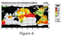
 Geographic distribution of the numbers of shells in the surface sediments (Figure 6) Geographic distribution of the numbers of shells in the surface sediments (Figure 6)
Map is based on a total of 11 reports, but over 85% of the data are from Goll and Bjørklund (1971, 1974) (Atlantic Ocean, 59% of the datapoints),
Bjørklund and Kruglikova (2003) (northern North Atlantic, 17%), and
Kruglikova (1966) (North Pacific, 9%). Since these figures are based on dried samples, where radiolarian shells have been shown to undergo sometimes significant destruction (Itaki and Hasegawa, 2000), the values depicted may be underestimated.
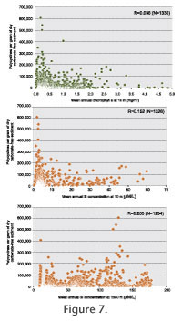
Shell concentrations in the sediments vs. mean annual chlorophyll a and dissolved Si (Figure 7)
Chlorophyll data are mean annual values at 10 m depth (from
Conkright et al. 1998a,
1998b,
1998c). Si data (mean annual values for 10 and 1500 m) are from
García et al. (2006). |