Material and methods

Altogether 348 samples are considered (Table 1). The majority (261) are from our previous studies (Figure 1). In addition, there are 55 new samples from southern England temperate brackish estuaries with bordering marshes (Christchurch and Poole Harbours, Beaulieu, Exe and Hamble estuaries), 25 from Norwegian fjords (shallow, 35-150 m: outer Lyngdalsfjord, Frierfjord, and Kragerø basin and outer Oslofjord; deeper than 400 m: Sørfjord, Hardangerfjord), four from the Skagerrak and three from the continental shelf Muck and Stanton deeps off Scotland (shelf deeps). All samples, representing the surface 1 or 2 cm of sediment, were stained with rose Bengal. In each case the >63µm living (stained), ODA and ATAs have been studied separately. The aim of acid treatment is to make it easier to pick sufficient agglutinated tests by removing the calcareous forms. The ATAs were prepared by dissolution in dilute acetic acid (pH 2.0-2.5). In the case of the deep fjord samples, the ODAs were rich in agglutinated tests so acid treatment was not necessary as sufficient tests could readily be picked. For consistency with the ODA data, ATA assemblages comprise dead tests only.

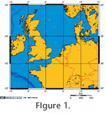
Tubular tests were not counted because they fragment during sampling and processing and give unreliable numbers. In some cases the multilocular test readily breaks into fragments (e.g., Reophax moniliformis, Hormosinella guttifer) so only those individuals with three or more chambers were counted towards the ATAs (following the practise of Murray and Alve 1999a).

Environmental data have been compiled from the sources listed in Table 1. In addition, the sea floor flux of organic matter has been calculated for shelf seas and the deep sea (see below). For shelf seas, all samples are from beneath areas of summer thermocline except for four samples from the southern North Sea (#3445, #3446, #3454, #3456). Fjords commonly have an estuarine water circulation but are distinguished from e.g., British estuaries by their silled basins, water stratification and sometimes by the presence of low oxygen or anoxic bottom waters. The examples here are all from oxic bottom water conditions.

Non-metric Multi-dimensional Scaling (MDS), principal component analysis, and species diversity calculations have been performed using Primer v.6.1.6 (Clarke and Gorley 2006). The MDS technique plots samples in two-dimensional space 'such that the relative distances apart of all points are in the same rank order as the relative dissimilarities (or distances) of the samples, as measured by some appropriate resemblance matrix calculated on the (possibly transformed) data matrix.' (Clarke and Gorley 2006, p. 75). For MDS the faunal data were transformed using square root and resemblances calculated using the Bray Curtis method. For the multivariate analysis (principal component analysis and MDS) of the abiotic factors plus sea floor organic flux the data were normalised prior to analysis. Species diversities have been calculated using Fisher alpha (Fisher et al. 1943) and the information function, H(S) (=H'(ln)), (Shannon 1948; Hayek and Buzas 1997).

Figure 1 was prepared from www.aquarius.ifm-geomar.de. Coloured images of species were taken using AxioVision Release 4.7.2 at the Natural History Museum, London. For each specimen, successive images were taken at different focal depths from the highest level downwards. These images were then merged using Auto-Montage 4.0 to give the sharpest image. The system works best on larger individuals, and it is difficult to achieve really sharp images of very small individuals. However, the results are images that show the natural colour and texture of the tests (although a few, such as Miliammina fusca, which was previously coated in gold, look more yellow than normal). The figures were compiled using Adobe Photoshop CS4. Some images show specimens stained with rose Bengal but such individuals were not included in the assemblage counts (based on dead only).

Sea Floor Organic Flux

Data on the average sea surface primary production per day are now available from satellite imagery (NEODASS) and from these data the annual rate is readily calculated. Primary production by plankton in the surface waters of the ocean and marginal seas is consumed by organisms as food or by bacterial decay during its descent through the water column. The amount of organic carbon that reaches the sea floor is termed the sea floor organic flux (Kaminski et al. 1999). In a classic study of the relationships between primary and export production, Berger et al. (1988) discussed previous attempts to quantify the downward flux of organic material and proposed various equations for its calculation at different water depths. They also concluded that the coastal regions of the oceans and sub-polar regions account for 50% of the total production and more than 80% of the flux of organic material to the sea floor. Altenbach et al. (1999) used Berger et al. equation 12 in their calculations of flux rates (F) for the eastern Atlantic Ocean. The factors are water depth in m (labelled z by Berger and D by Altenbach) and annual primary production (PP) as g C_org m^-2 yr^-1. Equation 12 is: F(D)=9PP/D + 0.7PP/D^0.5. An alternative equation (11) for shallower waters is J(z)=6.3*PP/z^0.8. However, the results differ by only 2-3% for water depths down to 200 m so, in the present study, equation 12 has been used throughout to calculate the C_org flux to the sea floor at investigated sites. In coastal areas the presence of suspended sediment causes the determination of PP to be less accurate so satellite data for these areas (A-L, Figure 1) have not been included. An example of this is found in Tilstone et al. (2005).

Data on average daily sea surface primary production are available for the years 1998 to 2005. For the shelf sea areas away from the influence of suspended sediment there is remarkably little variation in the pattern of values from one year to another. The 2005 data were used for this study. Rather than calculate the values for each precise data point a general value has been taken for each main area, shelf sea (M-V, Figure 1: North Sea Forties and Ekofisk, Skagerrak, outer Celtic Sea, Scotland shelf deeps all 146 g C_org m^-2 yr^-1; central Celtic Sea 219 g C_org m^-2 yr^-1) and for the deep sea (73 g C_org m^-2 yr^-1). However, for each sample the sea floor organic flux has been determined according to water depth using equation 12 as noted above. This general approach to determining sea floor organic flux is justified because the foraminiferal data represent an average of decades of foraminiferal accumulation so there is no point in making comparisons with a precise value based on a single observation of the sampling spot.

Although the primary production of coastal areas cannot be reliably determined due to the masking effects of suspended sediment, in such areas the main food source for benthic foraminifera is likely to be the benthic flora of diatoms, bacteria and cyanobacteria together with organic detritus derived from marine or terrestrial plants or degradation products. Whereas in shelf seas and deep sea areas the most variable environmental parameter is likely to be the sea floor organic flux, in shallow waters there is greater variation in abiotic factors such as temperature, salinity and energy from waves and/or water currents.

Taxonomy

Where necessary we have revised the taxonomy of our previous studies. Type material was examined in the Natural History Museum, London, and reference examples of 'Labrospira jeffreysii' (Williamson) and Trochamminella bullata Höglund were provided from the Höglund Collection in Aarhus University, Denmark. Altogether, there are 92 named agglutinated species. Notes on individual taxa are given in the taxonomic list.