Mapping the past

Mapping the past: GIS and intrasite spatial analyses of fossil deposits in paleontological sites and their applications in taxonomy, taphonomy and paleoecology

Gáspár Albert, Gábor Botfalvai, and Attila Ősi

Article number: 21.3.5T
https://doi.org/10.26879/812
Copyright Society for Vertebrate Paleontology, December 2018

Author biographies
Plain-language and multi-lingual abstracts
PDF version

Submission: 26 July 2017 . Acceptance: 29 November 2018

{flike id=2370}

ABSTRACT

At paleontological excavations, the use of digital surveying tools is becoming more frequent to measure the geographical location of specimens. This technology filtrates into the discipline of paleontology from archaeology, where the mapping methodology is quite similar, and the GIS as a standard tool for analysis is more widespread. The result of such a survey is a geodatabase, which forms the basis of subsequent analyses. The workflow is represented as the: 1) surveying, 2) database building, and 3) spatial analysis creating maps or 3D models. The presented methodological paper describes the details of the workflow, explaining the best practices and highlighting those issues which are necessary to be targeted even on the field. The methods tackle the optimal database structure, the spatial querying, which is managed from simple data table formats, and the 3D modelling. Explanations for these topics are given throughout specific programs; however, the tasks are also described generally enabling the reader to apply the described method to other programs. The data structure is explained through Excel worksheets, and for the analysis, an Excel-based macro script was developed, which is published as a supplementary material of this paper. Complex spatial analyses and visualization were done with Jewel Suite, a geological 3D modelling application. Demonstrating the workflow, three types of taphonomical inquiries are discussed using the surveyed materials of the Santonian dinosaur bed at the Iharkút site (Hungary). This technique is easily applied and becomes an important tool to obtain more precise taxonomical, taphonomical, and paleoecological interpretations in fossil excavations.

Gáspár Albert. Eötvös Loránd University, Department of Cartography and Geoinformatics, Pázmány Péter prom. 1/A, Budapest, 1117, Hungary. albert@ludens.elte.hu
Gábor Botfalvai. Hungarian Natural History Museum, Department of Palaeontology and Geology, Baross st. 13, Budapest, 1088, Hungary; Eötvös Loránd University, Department of Physical and Applied Geology, Budapest, Pázmány Péter prom. 1/C, Budapest, 1117, Hungary; and Eötvös Loránd University, Department of Paleontology, Pázmány Péter prom. 1/C, Budapest, 1117, Hungary. botfalvai.gabor@gmail.com
Attila Ősi. Hungarian Natural History Museum, Department of Palaeontology and Geology, Baross st. 13, Budapest, 1088, Hungary and Eötvös Loránd University, Department of Paleontology, Pázmány Péter prom. 1/C, Budapest, 1117, Hungary. hungaros@gmail.com

Keywords: bone mapping; paleontological database; 3D modelling; vertebrate taphonomy; spatial analyses; bonebed

Albert, Gáspár, Botfalvai, Gábor, and Ősi, Attila. 2018. Mapping the past: GIS and intrasite spatial analyses of fossil deposits in paleontological sites and their applications in taxonomy, taphonomy and paleoecology. Palaeontologia Electronica 21.3.5T 1-22. https://doi.org/10.26879/812
palaeo-electronica.org/content/2018/2370-mapping-the-past

Copyright: December 2018 Society of Vertebrate Paleontology.
This is an open access article distributed under the terms of the Creative Commons Attribution License, which permits unrestricted use, distribution, and reproduction in any medium, provided the original author and source are credited.
creativecommons.org/licenses/by/4.0/creativecommons.org/licenses/by-nc-sa/4.0/

INTRODUCTION

In vertebrate paleontology, mapping of specimens is a key activity during excavation, because the original positions of the buried fossils provide essential information about the depositional history of the bone concentration, and it cannot be reconstructed after removing the fossils from the bonebed. However, the mapping of specimens during the excavation is a time-consuming activity, and the building of a meter-grid system can be complicated in the case when the mapping is done on an irregular surface (e.g., Abler, 1984; Organ et al., 2003; Britt et al., 2009). Although putting the recorded data into a database and constructing digital maps make the process more complicated, a well-constructed digital map provides indispensable data that can be used to interpret the depositional conditions at the time the assemblage was concentrated and buried (Eberth et al., 2006; Jennings and Hasiotis, 2006).

From taphonomical aspects, recording the position, size, and orientation of fossil bones (referred as “bone mapping”) is especially informative. Over the last decades, our knowledge about the dispersal and depositional modes of the transported bone materials continuously increased due to several field and laboratory studies (e.g., Badgley, 1986b; Behrensmeyer, 1978; Dodson, 1973; Kaufmann et al., 2011; Lyman, 1994; Voorhies, 1969 and references therein). These works provide useful information about the preservation, transport, and burial of bones and other skeletal specimens, and can be applied to understand the processes which created the fossil bone concentrations.

Despite the growing taphonomical knowledge, the methodology and usability of the outcrop-scale fossil mapping has changed only in small increments during the last decades. The meter-grid system and the measuring tape (e.g., Alberdi et al., 2001; Eberth et al., 2006; Rogers, 1990) are still the most commonly used techniques for mapping specimens in paleontological sites, in spite of the more usable and more precise surveying devices modern surveying technology has developed (for example: total stations and geodesic GPS). These tools make it possible to quickly record the lateral and vertical position of all specimens with the same (or higher) precision, as the traditional metric grid can provide with a measuring tape. Either way, the positions of the collected elements are measured, and the spatial relations can be analyzed with programs if the data are recorded in a database.

The geographic information system (GIS) is a useful tool for analyzing the spatial distribution of the collected specimens. It consists of a database and a program (e.g., ArcGIS, QGIS, GRASS, MAPINFO), which can run queries and display the spatial data in a map form. Application of GIS is already widespread in archaeology for the very same purpose as it can be of use in paleontology: to help mapping specimens (Rayfield et al., 2005; McCoy and Ladefoged, 2009; Reed et al., 2015). It also helps to evaluate the mapping data in order to show relationships (using statistic methods) in the bone material, which remain hidden during visual interpretation. The importance of spatial technology in the interpretation of paleontological and archeological data has long been recognized and can be classified into three categories: data management, visualization, and spatial analysis (Harris and Lock, 1995; Goodchild et al., 1992; Breithaupt et al., 2004; Katsianis et al., 2008; McCoy and Ladefoged, 2009; Wheatley, 1995; Wheatley and Gillings, 2003; Anemone et al., 2011 and references there in). Also, several mapping techniques were developed characterizing the processes which influenced the formation of the excavated site (e.g., Jennings and Hasiotis 2006; Anderson and Burke, 2008; Benito-Calvo and de la Torre, 2011; Gallotti et al., 2011; de la Torre and Benito-Calvo, 2013; Bertog et al., 2014; Birkenfeld et al., 2015; Giusti and Arzarello, 2016 and reference there in). Archaeologists have already implemented quantitative methodologies in order to evaluate the measured data (e.g., Nigro et al., 2003; McPherron, 2005; McCoy and Ladefoged 2009; Anderson and Burke, 2008; Houshiar et al., 2015; Giusti and Arzarello, 2016 and references therein), but in paleontology these methods are infrequently applied, and researchers rather relied on the visual interpretation of bone distributions for the identification of spatial patterning within paleontological levels (Eberth et al., 2006). This phenomenon probably can be explained because the paleontological sites usually represent a broader time interval, and the sedimentological, taphonomical, and taxonomical data are more incomplete and less reliable for the quantitative analyses (Oheim, 2007). Yet, there are a few examples, where high-precision surveying devices were applied during the excavations, and the mapped data were evaluated by GIS and statistical software packages (e.g., ArcGIS, SAS, BDMP) in order to facilitate taphonomy studies (Alberdi et al., 2001; Bertog et al., 2014; Bramble et al., 2014; Jennings and Hasiotis, 2006; Lacruz et al., 2003), or fossil site predictions (Oheim, 2007). These paleontological examples do not include detailed descriptions about the implementation of statistical methods, but suggest that the use of GIS allows paleontologists to complete more accurate quantitative analyses of spatial relationships pertinent to taphonomic interpretation. Although, in the listed examples the authors refer to their approach as a 3D analysis, some of the cited software packages have only limited capacity in 3D spatial statistics (e.g., ArcGIS, ArcScene), projecting the 3D data on surfaces or planes. Thus, the spatial nature of the collected data could not be fully exploited. Methods of GIS based true 3D modelling, which exploits the spatial variables, may comprise explicit and implicit modelling (Maxelon et al., 2009). Explicit methods aim for a 3D representation of the measured data in a virtual environment in order to explain the outcrop geometry, stratigraphy, and orientation of the observed phenomena, from 3D aspects. The model is a result of iterative work processes, where the geometrical elements are placed deterministically in the virtual environment by the modeler manually or semi-automatically (Breunig, 1999; Kaufmann and Martin, 2008). Implicit modelling methods use the Euclidian coordinates (x, y, z) and the qualitative or quantitative attributes of the findings as geostatistical variables to produce estimations on the locations where measured data are not available (Breunig, 1999; Kaufmann and Martin, 2008).

In geosciences the explicit and implicit methods are usually combined with each other using the geodatabase of primitive (i.e., points, vectors) and complex (like surfaces, blocks) spatial structures; furthermore the analysis is not limited to surfaces or vertical planar sections (Calcagno et al., 2006; Jones et al., 2009). Instead, the program, which performs the spatial query, works with the tessellation of volumetric elements (volume pixels or voxels), the size of which define the spatial resolution of the model (Jessel, 2001). Each voxel usually has an hexahedral shape and is associated with a record in the background database containing several attributes. When such a modelling system is applied, one can perform multivariate statistical methods to estimate the unknown attributes of a spatial position (assigned to a voxel) using the geometry of the known locations (i.e., the voxels where measured data can be found). Depending on the used mathematics, the results will differ from each other, but all of them are considered as estimations inevitably bearing uncertainties (usually referred to as the error of the modelling method). The modelers’ responsibility is to select the method producing the smallest error.

The aim of the present study is to give an insight into the usability of the spatial analysis in fossil mapping and explain the methodology of the used programs. In contrast to the previously mentioned studies it explains the workflow of the whole process in details, which should be followed to build a working GIS from the recorded specimens. The geodatabase, and the modelling methods described in the paper are created to utilize them in the most common taphonomical analyses. Demonstrated by the 3D mapping of a bone-yielding bed of the Late Cretaceous vertebrate locality in Iharkút, Hungary, the presented methods allow the production of simultaneous or separate visualizations of the original data or the modelled results and analyses of the fossils within their original spatial contexts. They also permit intrasite spatial analyses that allow a comprehensive investigation of the site formation processes. Both traditionally measured and digitally surveyed data can be processed this way if the precision of the data makes it possible.

WORKFLOW OVERVIEW

Working with the collected paleontological data of an excavated site requires constructing an information system (analogue of a GIS), which has three main functionalities from the aspect of data management: 1) processing; 2) storing; and 3) representation. All of these functionalities (Table 1) are handled with different component programs, since such complex program suites do not exist for paleontological purposes yet. The component programs of the GIS must be able to communicate with each other via import-export file types or direct database connections. Although, using various programs makes the process complicated, the flexibility of the components allows one to create a workflow, which leads to the overall aim: a high resolution spatial model of the site with database background.

Such a workflow is presented here to facilitate the spatial analysis of paleontological data that have been measured either with traditional or modern surveying tools. It includes two component programs: Excel with Visual Basic scripts mainly for the processing and storing functionalities, and Jewel Suite modelling program for the visual representation. The result of the workflow is a GIS allowing one to create models and draw conclusions from the spatial analyses. The types of analyses are varying depending on the goal of the modeler, but basically taphonomical and taxonomical models can be derived from the data. However, the method is applicable only if the collected data were mapped and all the findings have spatial position measured with a precision of a few centimeters.

Measurement Processes at the Site

From the aspect of spatial analysis, mapping the exact position of bones and other findings at the site is crucial, because after removing the fossils their accurate positions are not available anymore. The planning of such activity should be defined stepwise to avoid loss of data. If taphonomical analysis from the findings is also planned, not only the fossils, but the layer boundaries (top/bottom) should be measured, along with the fossil’s vertical position relative to them. The findings overlaying each other in the beds obviously will have the same x, y (horizontal coordinates in a Cartesian system), so measuring only the horizontal geographical parameters is not enough; a third coordinate should be added (elevation or vertical distance from the top of the layer). Defining a Cartesian coordinate system at the site may occur physically (grid of ropes and spikes), or virtually (geodesic methods); also the two of them can be combined.

The meter-grid (box-grid) system is the most commonly used technique for mapping specimens in a quarry, and it can produce the proper resolution for GIS-based analyses. It is quite adequate if the site is flat and relatively small, and easy to record the locations of the findings by measuring their horizontal distances from the grid nodes (e.g., Abler, 1984; Botfalvai et al., 2017; Britt et al., 2009). However, this technique is an invasive method and involves several difficulties when paleontologists try to use it on rough terrain. For example: (1) the spikes hammered into the quarry floor as grid nodes can destroy the buried bones when beaten into the layer (Organ et al., 2003); (2) if the site is situated on a hillside or on uneven ground surface, building the grid is time-consuming and complicated; (3) measuring the vertical position of the findings is more problematic than measuring the horizontal coordinates. Although the invasiveness can be avoided with the “floating-gird” system presented by Chris L. Organ and his colleagues (Organ et al., 2003), it is even harder to set it up on steep slopes. Furthermore, the traditional meter-grid mapping method is unusable if the bonebed is expansive (several hundred meters long and wide) and its fossil-content is sparse and scattered.

Using high precision geodesic devices such as total stations (computerized theodolites), or real-time kinematic (RTK) GPS has already become widespread at archaeological and paleoanthropological excavations, gradually replacing the analogue meter-grid method (Neubauer, 2004; McPherron, 2005; Roosevelt et al., 2015; García-Moreno et al., 2016), but they are used only at a few paleontological sites (Bertog et al., 2014). Since the excavation techniques are quite similar in these disciplines, the modern surveying devices are of great use for paleontologists too, and the advantage of precise geolocation is already acknowledged in prospecting new sites (Anemone et al., 2011; Oheim, 2007). Although these methods are flexible enough to handle multiple approaches to excavation, and survey the position of fossils very quickly and easily without meter-grid system, both techniques have advantages and disadvantages. If total station is used, the surveying can be done even in covered sites (under a roof or inside a cave), but handling the instrument and the measuring rod requires two persons, and it takes 5-10 minutes to put a record correctly into the database. Measuring with an RTK GPS is quicker (it takes only 2-5 minutes to record one finding), and it is handled by one person, but it relies on the Global Navigation Satellite System (GNSS) and the GSM network, and thus, it can be used only in open areas. The precision of such surveying tools is within a few centimeters both horizontally and vertically, and after connecting them to a portable computer, the collected data can be processed even on the site. Using these surveying methods at excavations that are separated from each other, the uniform geodesic coordinates allow paleontologists to analyze the spatial relations of findings from multiple locations.

However, during a measurement one has to record several attributes of the fossil with the surveying device, if the overall goal is to create a complete database on the site.

Database Structure

The direct digital recording of observations at the time and location of actual excavation has a great priority, because the missed measurements are often irreplaceable after the excavation. Yet, the digital surveying procedure can be more time consuming than it is expected, extending the recording time of one single fossil with the description of several parameters (type, size, preservation, orientation, etc. see Supplementary 1). Slow surveying may halt the excavating process, so it is important to find the optimal data structure, which is detailed enough to contain the necessary information, but easy to record it quickly with the surveying device. Reed et al. (2015) address this problem as the main challenge of the piecewise mapping of fossils. They also provide recommendations for a paleoanthropological database standard (PaleoCore), which is built on free and open source technology. However, a database structure optimal for post processing (e.g., statistical analysis), is not always useable on the field.

The technical requirements of the surveying program, which runs on the used instrument, usually predefines the possibilities regarding the complexity of the data structure, but the overarching goal - to record it quickly - is common. The aim of the surveyor is to record as many pieces of information as possible in the shortest time, but the technique to achieve this can be different depending on the customizability of the surveying program running on the controller unit of the recording device; the following cases are the most common:

1. The program can handle multiple data fields and pre-defined dropdown lists, which help the surveyor to select the proper data types quickly.

2. The program handles several data fields but no dropdown lists.

3. The program can handle less data fields than the number of different data types, which are planned to be recorded.

The first is the optimal case, and there is a tendency that it will become widespread in the future. However, the second and third cases are common for most devices fabricated in the last two decades. To facilitate the recording, the usual method in these cases introduces abbreviations/codes (Table 2) for the data categories which can be quickly typed in even on the field.

The codes can be concatenated to each other when recording them, thus enabling one to use only one database field for different information. If the method was used properly, the different data types can be reconstructed easily from the reduced database after downloading them to a computer. Subsequently the separated data is uploaded into a relational database (RDB) as contents of separate data fields (columns). To set up and maintain a GIS such RDB is necessary to construct, because it will provide the source data for the spatial analyses.

Application of the Method in the Field

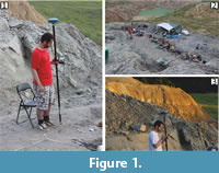During the excavation of the Late Cretaceous (Santonian) bonebed of the Iharkút vertebrate site (Hungary) (Ősi et al., 2012), in the summers of 2014-2016 a Spectra Epoch RTK GPS was used to record the position of fossils (Figure 1). Its controller PDA unit was equipped with Windows mobile platform and the customization of the data structure was limited, so reduction of different data types into one entry field - as described above - was necessary. All the teeth, bones, and coprolites were separately measured by their coordinates. In addition, any features of specimens (e.g., size, taxonomical position, and anatomy) were also documented along with their positional data (Supplementary 1). These characteristics were coded as numbers or as uniform abbreviations in the generated database. Furthermore, top and bottom of the bonebed layer were also measured in different points during the excavation in order to provide explicit information about the bonebed geometry.

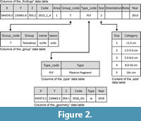
After three weeks of surveying, the database of the fossils was reconstructed in Excel and sorted into four data tables (worksheets): 1) records of all findings; 2) taxonomical groups; 3) anatomical types, and 4) size categories. Each year the database was updated with approximately 900 new measurements. The measurements of the stratigraphic unit’s top and bottom layer made up a fifth data table (Figure 2).

Evaluation of the Measured Data

The reconstructed database was simple enough to manage it in Excel, and most of the querying and summing tasks do not require special knowledge in data management. However, some of the spatial querying tasks made it necessary to create customized macros as part of the database file. Excel contains a script editor interface, which facilitates the writing of sub-routines (macros) and functions in Visual Basic programming language. The created program code will be an organic part of the Excel file and can be executed as a macro; though, one has to allow the program to open files with macros to reach this functionality.

The connection between the data tables was defined via the “IF” and the “LOOKUP” functions of Excel, and a few macro scripts. The macros were developed to run complex spatial queries in the database answering the following questions:

1. How many other - possibly similar - findings are located around the fossils of a given (or more) taxonomical group(s) within a defined buffer zone?

2. How many findings with similar/different anatomical types are located around a given (or more) taxonomical group(s) within a buffer zone?

3. What is the optimal resolution of a 3D grid model aimed to represent the spatial distribution of the findings?

Furthermore, the macros provided the connection to the 3D modelling component program (Jewel Suite) by formatting the query result into the proper data structure. The questions were answered with lists of fossils (identifiable by their ID code) and statistical data which can be visualized on maps and diagrams.

Data analysis within the Database

The database of the Iharkút vertebrate site between 2013 and 2016 contains 3892 records in the “findings” table (Supplementary 1). The geographic positions are defined in the Hungarian National Grid System (Mihály, 1996), which has served as the Cartesian coordinate system for the measurements. The taxonomical groups were defined into 30 and the anatomical types into 56 categories (see “type” worksheet in Supplementary data 1). The categorization of groups does not follow the taxonomical hierarchy because identification of a finding on the site depends on the preservation and preparation conditions of the fossil. The level of uncertainty is reflected in the use of “one fits for all” categories like Sauropsida (S) or even Vertebrata (V). Categories like this were also used describing uncertain anatomical types (e.g., bone as B).

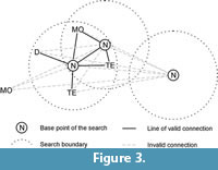When analyzing such diverse data, one has to consider the possibility that some of the differently identified specimens can belong to the same - usually more specified - taxa, and even to the same carcass amongst the scattered remnants. The goal is to find out whether the well-defined findings can help to identify the fossils which may belong to the same carcass by running complex spatial queries on the database (Figure 3). Subsequently, the queried group of findings can be re-analyzed thoroughly. Such data analysis was handled with a macro (Supplementary 1; GroupSelect) in the Excel file, which initialized a query form (Figure 4).

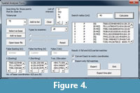The form offers a multi-select list of taxonomical groups and the filtering option for specific anatomical types. Taxonomical groups can be selected as the geometrical base of the spatial search, and also a search list can be created from (different) groups. The script will look for the findings, which are in the search list and located within a specified buffer distance from the findings, defined as the geometrical base of the search. Using the form, one can work with external coordinate files too, allowing specifying locations of high interest manually as the geometric base of the query.

The result of a query can be exported as a new data table in column separated .txt file format (Table 3). The columns of this table are the followings: finds; findType; Code_list; Xm; Ym; Zm; Code(base); Code(finds). The detailed description of the file structure is given in the supplementary documentation (Supplementary 2).

Also, the query result can be exported as a 3D line-plot, which is of use in the visualization of the associated findings (i.e., as a map). The file format is .bln (simple ASCII type), which can be imported into standard GIS programs.

Working with the Data in a 3D Modelling Environment

The familiar user interface of Excel made it possible to run spatial queries by paleontologists untrained in database management and study the properties of the results by numbers. However, the visual representation of the results was not available within this component program. For visualizing, and analyzing the results of the spatial queries, or the whole database, a different component program - JewelSuite (JS) - was used, which is capable of creating 3D stratigraphic and parametrized models. Furthermore, this program was capable to combine the results of the spatial querying with the explicit modelling methods based on the geometry measurements of the bonebed.

This component program is a full workflow framework that supports and describes every step needed to build complex 3D geological models (BakerHughes, 2017). The files are called “solutions” as they represent only one of the many solutions of a problem (like ‘where can I find the places which are within 30 cm from a certain type of object?’). When starting a new project in JS, one has to create and save a project file with an extension .jewel. This file contains the database and all the user settings associated with a given project, and when opening a .jewel solution file, one has access to all the geometric and parametric data stored in the database.

Although the program has its advantages in using built-in measurement units that can be converted from one to another easily, it is not designed to create models with a few centimeter resolutions. The processed Iharkút bonebed RDB was measured almost on sub-centimeter resolution with the RTK GPS. To avoid unwanted upscaling during modelling, the meter-based coordinate geometrical data was transformed to represent centimeters as base units prior to importing it into JS as meters. This was achieved with a trim of large numbers from the Easting, Northing, and elevation data and multiplying the result with one hundred. Additionally, since in JS the Z-axis in the modelling environment points downward and is called tvss (true vertical subsea depth), the elevation values were switched to negatives.

With the modelling program, the database of fossils is visualized in the 3D environment, and even this may help the paleontologists to understand spatial relations amongst the findings. For example selecting one or a few taxonomical groups to be visualized and hiding the others may reveal clusters of findings, triggering taphonomical insights. Using this basic functionality is not an act of real spatial modelling in a sense that new data are not created by mathematical methods. Modelling actions - creating estimations with the component program - can be the following in this sense:

1. New property is created for an already existing object using existing ones (e.g., geometry data is queried for the points containing their distance from the top and/or bottom layer of the bonebed).

2. Entity with higher complexity is created from base data having lower complexity (e.g., surface model from dispersed points, or volumetric model in between surfaces and/or around dispersed points).

Properties of an object are basically imported into the modelling program with the original database (like the codes of the taxonomical groups, the anatomical types, or the year of finding). The importing process, however, creates a copy of the original database, which can be extended with new fields (columns) but not connected anymore to the original database. The new properties are created via the Property Calculator sub-application of the modelling program.

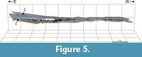The surface modelling is based on the measurements of the top and bottom layer of the bonebed. The records of the “geometry” data table are imported into the modelling program and models for the base and the top boundary surfaces are created via interpolation (Figure 5). The surface geometry can be a network of irregular triangles (TIN model) or a regular grid; the surface modelling method is an important element of the process, which has to be selected for the specific situation to achieve the minimum errors (Yang et al., 2004).

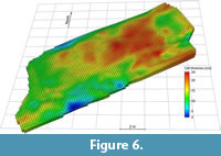
With the volumetric modelling, one specifies a void (modelling area) where the program will calculate estimations for those places where direct observations were not present. These calculations are usually interpolations and geostatistical estimating processes. It is also called implicit modelling (Calcagno et al., 2006). The model is composed of small tessellated cell units (voxels) each of them having their own (estimated or measured) properties. The size of these units specifies the 3D resolution of the model, and their shape is most often hexahedral (Figure 6). The center points of the cells - forming a spatial grid - are defined as individual database records (rows in the data table). The volumetric model also gives information about the physical extent of the processed materials in cubic meters.

Both the surface and the volumetric modelling produce new geometry (exactly defined points of the surface and the voxels) in the modelling environment, which must be handled almost similarly as the records of the original database. This can be done only if the modelling program (such as the JS) is capable for GIS operations. In this case further analysis can be done in the modelling program. Alternatively the data of the new geometry (records of the grid nodes) are exported into a new database and are analyzed by the modeler using the functionality of an external program. Such possibility is also given in the workflow presented here, if one wishes to use the Excel macro with a text-type database file.

Calculating the Optimal Resolution of the 3D Model

The resolution of a volumetric model plays a primary role in the geostatistical processes. If too large cells are used (e.g., larger than the thickness of the bonebed), the varying original records will be averaged, and the most occurring parameters will dominate the results. On the other hand, if the cells of the model are too small, one original record will affect too many cells, creating unnecessary duplications. Furthermore, large resolution slows down the calculation processes, so it is best to avoid creating unnecessarily small voxels.

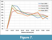The optimal size of the grid resolution was calculated from the original database records using the Excel macro (GroupSelect) to create groupwise spatial queries. The following analysis created several new column-based data table as the result of the queries, each of them representing the number of findings around the points of the selected taxonomical group in a defined buffer distance. These files contained the numbers of query matches in the “finds” column. With the repeated search of similar categories by modifying the search radius around the individual points of a specific taxonomical group from 10 to 100 cm with 10 cm intervals, one can compare the query matches (the database-files) to find an abrupt increase of the numbers. The initial value was one (since the center of the search was the first of the finds); those occurrences were counted where the increase of similar taxa was doubled relative to the previous interval (Figure 7). Using the richest bonebed of the Late Cretaceous Iharkút vertebrate locality (site SZ-6, see Botfalvai et al., 2015) as a case study, three taxonomical groups and the coprolites - having more than 600 records - were analysed, and the 10-20 cm interval which contained the most numerous “doublings” was selected as the cell size in the 3D grid. The interval distance is measured in all directions from the central node, making the possible cell size range 20-40 cm. As the smallest within this range, a 20 cm optimal grid resolution was selected for the 3D models. The vertical resolution, however, is varying between 2 and 24 cm (Figure 6); for this the defining parameters were the total thickness of the bonebed and the number of internal layers. The analyzed taxonomical groups were the Nodosauridae,Testudines and the Sauropsida; the latter represents all those findings, which were not determined on the site more precisely.

UTILIZATION OF THE WORKFLOW MODEL

In the following subchapter, we introduce three different taphonomical inquiries related to the richest bone bed of the Late Cretaceous vertebrate site in Iharkút, western Hungary (Ősi et al., 2012), which can be done by using the component programs and standard GIS applications described in the previous sections. The first of these tackles the general spatial distribution of fossil content. The second one concentrates only on the bone materials and tackles the size distribution both horizontally and in the vertical profile of the bone bed. The third one concentrates on the probability of association among the fossil remains. The goal of this subchapter is to introduce the possibilities connected to the abovementioned workflow model, but the interpretation of these results for the Iharkút site will be summarized in a further manuscript focusing on the depositional mode of the vertebrate material (see Ősi et al., in press).

The Iharkút vertebrate locality, an open-pit mine in the Bakony Mountains (western Hungary), has provided a rich and diverse assemblage of Late Cretaceous (Santonian) continental vertebrates (Ősi et al., 2012). The isolated and associated remains represent at least 35 different taxa including fish, amphibians, turtles, mosasaurs, lizards, pterosaurs, crocodilians, dinosaurs, and birds. Sedimentological investigations by Botfalvai et al. (2016) pointed out that the fossil-bearing Csehbánya Formation in Iharkút has been deposited by an anastomosing fluvial system in a topographically low-level, wet, alluvial plain environment. The most important fossiliferous layer in the open-pit mine is a 10-50 cm thick bonebed of site SZ-6, which was deposited during ephemeral high density flash-flood events probably triggered by episodic heavy rainfalls. The taphonomical investigations of the site SZ-6 were already conducted by Botfalvai et al. (2015). This work was based on the findings excavated earlier than the detailed GIS survey has started in 2014. The taphonomical analysis of the detailed survey is in progress, but as case studies, the major processes, involving the GIS technique mentioned above, are described in the followings.

General Distribution of Fossil Content in 3D

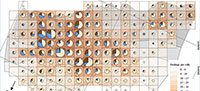
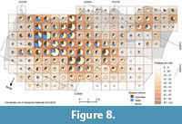
While a traditional bone map - depicting an excavation site - may give an overview of the distribution pattern, true spatial analysis can be done only within a spatial database, where the findings have absolute (measured) and relative height attributes (calculated). Instead of simply using the measured elevation data, one can apply the theory of the “law of superposition” in the taphonomical analysis by using the relative positions of the findings. In our workflow model, this parameter is calculated in the JS modelling program using the modelled base surface. The result is exported as a text file from the modelling program. It represents an enhancement of the original database (Supplementary 1), because two new columns (data fields) are added to the “findings” table (distFromBase and bedThickness). The first contains the distances of all findings from the base layer, and the second indicates the local thickness of the bonebed for each finding. These attributes can be used in conventional GIS programs such as ArcGIS, Mapinfo or QGIS to analyze the data. The result of such analysis can be represented as different maps of the whole bed (Gallotti et al., 2011). 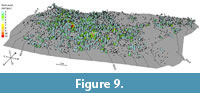For example, the functionality of the QGIS 2.12 program was used to calculate the point density in each cell using point- and area-type features respectively (Figure 8). Furthermore, using the relative position data, maps for different vertical zones (inner layers) within the bonebed, can also be created.

The JS modelling program also provide tools for calculating the density of findings (Figure 9). These calculations are applied on the fine (20 by 20 cm horizontal, and 14.2 cm mean vertical) resolution of the 3D model, which is created in the modelling environment.

The Distribution of Differently Sized Bones

The investigation of the size distribution of the bone material can answer the research questions, which are focusing on the sedimentation of the bone-bearing materials, since the bones behave as discrete sedimentary particles and thus they become sorted by size, shape, and density (Aslan and Behrensmeyer, 1996; Behrensmeyer, 1975). Several empirical observations were conducted in laboratories in order to determine the dispersal potential of different bone elements (Behrensmeyer, 1975; Coard and Dennell, 1995; Dodson, 1973; Kaufmann et al., 2011; Voorhies, 1969). 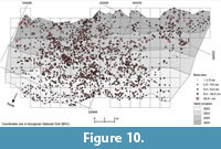Their results indicate that this sorting pattern refers to transport conditions and that the size, shape, and density of bones are key factors during the transportation. The vertical and horizontal distribution of different types of bones are varying according to the physical properties of the bonebed, and thus, the variations in depositional processes are best demonstrated in three dimensions to establish the relative changes across the site (Anderson and Burke, 2008; Bamforth et al., 2005; Britt et al., 2009; Gallotti et al., 2011).

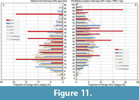
Using a standard GIS program and the original database, the horizontal size distribution can be represented as a map (Figure 10) without using the 3D modelling component program or the Excel macro, because the database of the Iharkút bonebed contained the necessary attributes for such analysis (size and type tables - see Figure 2). However, the analysis of the vertical distribution, or creating maps of certain layers of the bonebed, requires the additional relative position data (“distFromBase” and “bedThickness” fields), which were generated with the spatial modelling component program (JS) and exported as new attributes of the bone material into the database (see previous chapter). The analysis of the vertical distribution can be completed using Excel (Figure 11). Due to the varying thickness of the bonebed, the relative positions were the most informative, when only the thicker (>50 cm, see Figure 5) part of the bonebed was analyzed.

Analysis of Associations among the Findings

The 3D depiction of the spatial distribution of bones can clarify whether there are potential associations among elements, especially when multiple animals are present and represented by broken and disarticulated remains (Eberth et al., 2007). The degree of articulation in a bonebed is generally estimated in a qualitative sense (e.g., partially articulated) based on individual observations, while the probability of association of isolated skeletal elements is considered zero as long as there is no evidence for the probability of association among the vertebrate remains (Badgley, 1986a). However, degree of element association in a bonebed can be gauged in a qualitative fashion by evaluating the spatial proximity of bones in relation to original anatomic association (Eberth et al., 2007). Such spatial analysis can be executed on a geodatabase of the findings, and the results (as maps or 3D line plots) highlight the relationships of vertebrate remains.

The association pattern depends on different factors: i) the specified taxa as the base of the search, ii) the specified taxa as the target of the search, and iii) the defined buffer distance where the targets are searched. To quantify the probability of associations, a few already connected findings can provide the control data. The links between the associated findings are ranked by their proportion to the control distances. The analysis of the association pattern can be followed by a subsequent physical examination of the concerning materials.

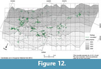Measurement of probability of association of isolated skeletal elements can also help in those cases when we want to connect different undetermined elements with well-defined cranial or mandibular elements. For example, four different taxa of Mesoeucrocodylia are documented based on cranial elements and tooth morphology within the Iharkút vertebrate assemblage (Ősi et al., 2012; Rabi and Sebők, 2015). However, mesoeucrocodylian postcranial elements from the same site cannot be easily assigned to any taxon, because their conservative morphology prevents the recognition of taxon-specific characters. In this case, the analysis of the association-patterns within the data can be a key tool to reveal certain connections between the cranial and postcranial elements of a single crocodyliform taxon (Figure 12).

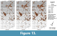
With the changing of the search radius, a dynamic variation of line-pattern is also informative, regarding the possible location of carcasses (Figure 13). Such dynamical analysis can be performed with the iterative querying of the database using the GroupSelect macro.

CONCLUSION

The demonstrated methods are new in a sense that such a spatial analysis has not been applied in taphonomical studies yet. Our aim was to create detailed documentation of this analysis to provide a workflow model. Although, parts of the workflow are available in 2D programs for GIS purposes, the tackled taphonomical inquiries are better executed in 3D in the demonstrated way. Without a 3D model, the spatial analysis of the bonebed is problematic because the relative position of the findings cannot be calculated and using only the elevation is not enough. In the workflow, we defined the optimal database structure, which included the physical measuring of the fossil-bearing strata. A base- and top-layer model - based on GPS measurements - was used in Jewel Suite to calculate the relative position of each fossil. Although, the presented JS modelling program provides easily executable solution for this, it is obvious that alternative methods (e.g., other modelling programs) can provide the same results.

Also, a significant part of the workflow was designed to exclude specialized commercial programs and to be manageable for those paleontologists, who got used to storing their data in simple table format (i.e., Excel). The developed VBA macro (GroupSelect) is optimized for Excel 2010 (v. 14) and newer. It helps to run complex spatial queries and exports the results in simple text format. Even those who have no access to JS (or similar 3D programs) can benefit from the database management and interpret the results on 2D maps. In the presented utilizations, such results were visualized with the QGIS open source 2D GIS application. The emphasis of the presented methods was on the stepwise process which results in maps, distribution diagrams, and 3D models from the database.

The new technique, presented here, can be an easily applicable method accessing paleontological field work. Results of these analyses can abruptly increase taphonomical data, help in clarifying taxonomical assignments of questionable but related fossil elements, and, in general, widen and help to visualize our interpretation in palaeoecological reconstructions.

ACKNOWLEDGEMENTS

We thank the anonymous reviewers for their useful suggestions and Zs. Koritár for the linguistic revision. Thanks to R. Kalmár (Hungarian Natural History Museum, Budapest) for technical assistance both on the field and in the collection. We are grateful to J. Mészáros, Z. Konrádi, and V.F. Kiss (Eötvös Loránd University, Department of Cartography and Geoinformatics, Budapest) for their technical assistance during measuring the bones. We thank the 2013-2016 field crews for their assistance in the fieldwork. We are grateful to the Bakony Bauxite Mines and to Geovolán Zrt. for their logistic help. Field and laboratory work was supported by the Hungarian Natural History Museum, the National Geographic Society (Grant Nos. 7228-02, 7508-03), the Hungarian Scientific Research Fund of the National Research, Development and Innovation Office (OTKA T-38045, PD 73021, NF 84193, K 116665), and the Hungarian Oil and Gas Company (MOL). This project was supported by the MTA-ELTE Lendület Program (Grant no. 95102), the Jurassic Foundation, and the Hungarian Dinosaur Foundation. The project was also supported by the ÚNKP-17-3 New National Excellence Program of the Ministry of Human Capacities.

REFERENCES

Abler, W.L. 1984. A three-dimensional map of a paleontological quarry. Rocky Mountain Geology, 23:9-14

Alberdi, M.T., Alonso, M.A., Azanza, B., Hoyos, M., and Morales, J. 2001. Vertebrate taphonomy in circum-lake environments: three cases in the Guadix-Baza Basin (Granada, Spain). Palaeogeography Palaeoclimatology Palaeoecology, 165:1-26. https://doi.org/10.1016/S0031-0182(00)00151-6

Albert, G. 2017. Aspects of cave data use in a GIS, p. 25-44. In Karabulut, S. and Cinku, M.C. (eds.), Cave Investigations, Intech, Rijeka. https://doi.org/10.5772/intechopen.68833

Anderson, K.L. and Burke, A. 2008. Refining the definition of cultural levels at Karabi Tamchin: a quantitative approach to vertical intra-site spatial analysis. Journal of Archaeological Science, 35:2274-2285. https://doi.org/10.1016/j.jas.2008.02.011

Anemone, R., Emerson, C., and Conroy, G. 2011. Finding fossils in new ways: An artificial neural network approach to predicting the location of productive fossil localities. Evolutionary Anthropology: Issues, News, and Reviews, 20:169-180. https://doi.org/10.1002/evan.20324

Aslan, A. and Behrensmeyer, A.K. 1996. Taphonomy and time resolution of bone assemblages in a contemporary fluvial system: the East Fork River, Wyoming. Palaios, 11:411-421. https://doi.org/10.2307/3515209

Badgley, C. 1986a. Counting individuals in mammalian fossil assemblages from fluvial environments. Palaios, 1:328-338. https://doi.org/10.2307/3514695

Badgley, C. 1986b. Taphonomy of mammalian fossil remains from Siwalik rocks of Pakistan. Paleobiology, 12:119-142. https://doi.org/10.1017/S0094837300013610

BakerHughes. 2017. JewelSuite Geologic Modeling. https://www.bakerhughes.com (accessed July 17, 2017).

Bamforth, D.B., Becker, M., and Hudson, J. 2005. Intrasite spatial analysis, ethnoarchaeology, and Paleoindian land-use on the Great Plains: the Allen site. American Antiquity, 70(3):561-580. https://doi.org/10.2307/40035314

Behrensmeyer, A.K. 1975. The taphonomy and paleoecology of Plio-Pleistocene vertebrate assemblages east of Lake Rudolf, Kenya. Bulletin of the Museum of Comparative Zoology at Harvard University, 146:473-578

Behrensmeyer, A.K. 1978. Taphonomic and ecologic information from bone weathering. Paleobiology, 4:150-162. https://doi.org/10.1017/S0094837300005820

Benito-Calvo, A. and de la Torre, I. 2011. Analysis of orientation patterns in Olduvai Bed I assemblages using GIS techniques: Implications for site formation processes. Journal of Human Evolution, 61:50-60. https://doi.org/10.1016/j.jhevol.2011.02.011

Bertog, J., Jeffery, D.L., Coode, K., Hester, W.B., Robinson, R.R., and Bishop, J. 2014. Taphonomic patterns of a dinosaur accumulation in a lacustrine delta system in the Jurassic Morrison Formation, San Rafael Swell, Utah, USA. Palaeontologia Electronica, 17.3.36A: 1-19. https://doi.org/10.26879/372
https://palaeo-electronica.org/content/2014/811-taphonomy-of-the-morrison-fm

Birkenfeld, M., Avery, M.D., and Horwitz, L.K. 2015. GIS virtual reconstructions of the temporal and spatial relations of fossil deposits at Wonderwerk Cave (South Africa). The African Archaeological Review, 32: 857-876. https://doi.org/10.1007/s10437-015-9209-4

Botfalvai, G., Haas, J., Bodor, E. R., Mindszenty, A., and Ősi, A. 2016. Facies architecture and palaeoenvironmental implications of the upper Cretaceous (Santonian) Csehbánya formation at the Iharkút vertebrate locality (Bakony Mountains, Northwestern Hungary). Palaeogeography, Palaeoclimatology, Palaeoecology, 441:659-678. https://doi.org/10.1016/j.palaeo.2015.10.018

Botfalvai, G., Ősi, A., and Mindszenty, A. 2015. Taphonomic and paleoecologic investigations of the Late Cretaceous (Santonian) Iharkút vertebrate assemblage (Bakony Mts, Northwestern Hungary). Palaeogeography, Palaeoclimatology, Palaeoecology, 417: 379-405. https://doi.org/10.1016/j.palaeo.2014.09.032

Botfalvai, G., Csiki-Sava, Z., Grigorescu, D., and Vasile, Ş. 2017. Taphonomical and palaeoecological investigation of the Late Cretaceous (Maastrichtian) Tuştea vertebrate assemblage (Romania; Haţeg Basin)—insights into a unique dinosaur nesting locality. Palaeogeography, Palaeoclimatology, Palaeoecology, 468:228-262. https://doi.org/10.1016/j.palaeo.2016.12.003

Bramble, K., Burns, M.E., and Currie, P.J. 2014. Enhancing bonebed mapping with GIS technology using the Danek Bonebed (Upper Cretaceous Horseshoe Canyon Formation, Alberta, Canada) as a case study. Canadian Journal of Earth Sciences, 51:987-991. https://doi.org/10.1139/cjes-2014-0056

Breithaupt, B.H., Matthews, N.A., and Noble, T.A. 2004. An integrated approach to three-dimensional data collection at dinosaur tracksites in the Rocky Mountain West. Ichnos, 11 (1-2):11-26. https://doi.org/10.1080/10420940490442296

Breunig, M. 1999. An approach to the integration of spatial data and systems for a 3D geo-information system. Computers & Geosciences, 25:39-48. https://doi.org/10.1016/S0098-3004(98)00104-6

Britt, B.B., Eberth, D.A., Scheetz, R.D., Greenhalgh, B.W., and Stadtman, K.L. 2009. Taphonomy of debris-flow hosted dinosaur bonebeds at Dalton Wells, Utah (Lower Cretaceous, Cedar Mountain Formation, USA). Palaeogeography Palaeoclimatology Palaeoecology, 280:1-22. https://doi.org/10.1016/j.palaeo.2009.06.004

Calcagno, P., Courrioux, G., Guillen, A., Fitzgerald, D., and McInerney, P. 2006. How 3D implicit geometric modelling helps to understand geology: The 3DGeoModeller methodology. XI. International Congress, Université de Liège, Belgium, Society for Mathematical Geology, S14-06.

Coard, R. and Dennell, R. 1995. Taphonomy of some articulated skeletal remains: transport potential in an artificial environment. Journal of Archaeological Science, 22:441-448. https://doi.org/10.1006/jasc.1995.0043

Deutsch, C.V. 1998. Cleaning categorical variable (lithofacies) realizations with maximum a-posteriori selection. Computers & Geosciences, 24:551-562. https://doi.org/10.1016/S0098-3004(98)00016-8

de la Torre, I. and Benito-Calvo, A. 2013. Application of GIS methods to retrieve orientation patterns from imagery; a case study from Beds I and II, Olduvai Gorge (Tanzania). Journal of Archeological Science, 40: 2446-2457. https://doi.org/10.1016/j.jas.2013.01.004

Dodson, P. 1973. The significance of small bones in paleoecological interpretation. Rocky Mountain Geology, 12:15-19

Eberth, D., Shannon, M., and Noland, B. 2007. A bonebeds database: classification, biases, and patterns of occurrence, p. 103-219. In Rogers, R.R., Eberth, D.A., and Fiorillo, A.R. (eds.), Bonebeds: Genesis, Analysis, and Paleobiological Significance. University of Chicago Press, Chicago.

Eberth, D.A., Britt, B.B., Scheetz, R., Stadtman, K.L., and Brinkman, D.B. 2006. Dalton Wells: Geology and significance of debris-flow-hosted dinosaur bonebeds in the Cedar Mountain Formation (Lower Cretaceous) of eastern Utah, USA. Palaeogeography Palaeoclimatology Palaeoecology, 236:217-245. https://doi.org/10.1016/j.palaeo.2005.11.020

Gallotti, R., Mohib, A., El Graoui, M., Sbihi-Alaoui, F., and Raynal, J. 2011. GIS and intra-site spatial analyses: an integrated approach for recording and analyzing the fossil deposits at Casablanca prehistoric sites (Morocco). Journal of Geographic Information System, 3:373-381. https://doi.org/10.4236/jgis.2011.34036

García-Moreno, A., Smith, G.M., Kindler, L., Pop, E., Roebroeks, W., Gaudzinski-Windheuser, S., and Klinkenberg, V. 2016. Evaluating the incidence of hydrological processes during site formation through orientation analysis. A case study of the middle Palaeolithic Lakeland site of Neumark-Nord 2 (Germany). Journal of Archaeological Sciences: Reports, 6:82-93. https://doi.org/10.1016/j.jasrep.2016.01.023

Giust, D. and Arzarello, M. 2016. The need for a taphonomic perspective in spatial analysis: Formation processes at the Early Pleistocene site of Pirro Nord (P13), Apricena, Italy. Journal of Archaeological Science: Reports, 8:235-249. https://doi.org/10.1016/j.jasrep.2016.06.014

Goodchild, M., Haining, R., and Wise, S. 1992. Integrating GIS and spatial data analysis: Problems and possibilities. International Journal of Geographical Information System, 6(5):407-423. https://doi.org/10.1080/02693799208901923

Harrish, T.M. and Lock, G.R. 1995. Toward and evaluation of GIS in European archaeology: the past, present and futures of theory and applications, p. 349-365. In Lock, G.R. and Stancic, Z. (eds.), Archaeology and Geographical Information System: A European Perspective. Taylor and Francis, London.

Houshiar, H., Borrmann, D., Elsberg, J., Nüchter, A., Näth, F., and Winkler, S. 2015. Castle3D—a computer aided system for labelling archaeological excavations in 3D. ISPRS Annals of the Photogrammetry, Remote Sensing and Spatial Information Sciences, 2(5):111-118.

Jennings, D.S. and Hasiotis, S.T. 2006. Taphonomic analysis of a dinosaur feeding site using geographic information systems (GIS), Morrison Formation, southern Bighorn Basin, Wyoming, USA. Palaios, 21:480-492. https://doi.org/10.2110/palo.2005.P05-062R

Jessel, M. 2001. Three-dimensional geological modelling of potential-field data. Computers & Geosciences, 27:455-465. https://doi.org/10.1016/S0098-3004(00)00142-4

Jones, R.R., McCaffrey, K.J.W., Clegg, P., Wilson, R.W., Holliman, N.S., Holdsworth, R.E., and Imber, J. and Waggott, S. 2009. Integration of regional to outcrop digital data: 3D visualisation of multi-scale geological models. Computers & Geosciences, 35:4-18. https://doi.org/10.1016/j.cageo.2007.09.007

Katsianis, M., Tsipidis, S., Kotsakis, K., and Kousoulakou, A. 2008. A 3D digital workflow for archaeological intra-site research using GIS. Journal of Archaeological Science, 35:655-667. https://doi.org/10.1016/j.jas.2007.06.002

Kaufmann, C., Gutiérrez, M.A., Álvarez, M.C., González, M.E., and Massigoge, A. 2011. Fluvial dispersal potential of guanaco bones (Lama guanicoe) under controlled experimental conditions: the influence of age classes to the hydrodynamic behavior. Journal of Archaeological Science, 38:334-344. https://doi.org/10.1016/j.jas.2010.09.010

Kaufmann, O. and Martin, T. 2008. 3D geological modelling from boreholes, cross-sections and geological maps, application over former natural gas storages in coal mines. Computers & Geosciences, 34:278-290. https://doi.org/10.1016/j.cageo.2007.09.005

Lacruz, R., Ungar, P., Hancox, P.J., Brink, J.S., and Berger, L.R. 2003. Gladysvale: fossils, strata and GIS analysis. South African Journal of Science, 99:283-285

Lyman, R.L. 1994. Relative abundances of skeletal specimens and taphonomic analysis of vertebrate remains. Palaios, 9:288-298. https://doi.org/10.2307/3515203

Maxelon, M., Renard, P., Courrioux, G., Braendli, M., and Mancktelow, N. 2009. A workflow to facilitate three-dimensional geometrical modelling of complex poly-deformed geological units. Computers & Geosciences, 35:644-658. https://doi.org/10.1016/j.cageo.2008.06.005

McCoy, M.D. and Ladefoged, T.N. 2009. New developments in the use of spatial technology in archaeology. Journal of Archaeological Research, 17:263-295. https://doi.org/10.1007/s10814-009-9030-1

McPherron, S.J.P. 2005. Artifact orientations and site formation processes from total station proveniences. Journal of Archaeological Science, 32:1003-1014. https://doi.org/10.1016/j.jas.2005.01.015

Mihály, S. 1996. Description directory of the Hungarian geodetic references. GIS, 4:30-34

Neubauer, W. 2004. GIS in archaeology—the interface between prospection and excavation. Archaeological Prospection, 11:159-166. https://doi.org/10.1002/arp.231

Nigro, J.D., Ungar, P.S., de Ruiter, D.J., Berger, L.R. 2003. Developing a geographic information system (GIS) for mapping and analysing fossil deposits at Swartkrans, Gauteng Province, South Africa. Journal of Archaeological Science, 30:317-324. https://doi.org/10.1006/jasc.2002.0839

Oheim, K.B. 2007. Fossil site prediction using geographic information systems (GIS) and suitability analysis: The Two Medicine Formation, MT, a test case. Palaeogeography Palaeoclimatology Palaeoecology, 251:354-365. https://doi.org/10.1016/j.palaeo.2007.04.005

Organ, C.L., Cooley, J.B. and Hieronymus, T.L. 2003. A non-invasive quarry mapping system. Palaios, 18:74-77. https://doi.org/10.1669/0883-1351(2003)018<0074:ANIQMS>2.0.CO;2

Ősi, A., Rabi, M., Makádi, L., Szentesi, Z., Botfalvai, G., and Gulyás, P. 2012. The Late Cretaceous continental vertebrate fauna from Iharkút, western Hungary: a review. Bernissart Dinosaurs and Early Cretaceous Terrestrial Ecosystems. Indiana University Press, Bloomington, Indiana, 532-569.

Ősi, A., Botfalvai, G., Albert, G. and Hajdu, Zs. in press. The dirty dozen: Taxonomical and taphonomical overview of an unique ankylosaurian (Dinosauria: Ornithischia) assemblage from the Santonian Iharkút locality, Hungary. Palaeobiodiversity and Palaeoenvironments.

Rabi, M. and Sebők, N. 2015. A revised Eurogondwana model: Late Cretaceous notosuchian crocodyliforms and other vertebrate taxa suggest the retention of episodic faunal links between Europe and Gondwana during most of the Cretaceous, Gondwana Research, 28:1197-1211. https://doi.org/10.1016/j.gr.2014.09.015

Rayfield, E. J., Barrett, P.M., McDonnell, R.A., and Willis, K.J. 2005. A geographical information system (GIS) study of Triassic vertebrate biochronology. Geological Magazine, 142(4), 327-354. https://doi.org/10.1017/S001675680500083X

Reed, D., Barr, W.A., Mcpherron, S.P., Bobe, R., Geraads, D., Wynn, J. G., and Alemseged, Z. 2015. Digital data collection in paleoanthropology. Evolutionary Anthropology: Issues, News, and Reviews, 24(6):238-249. https://doi.org/10.1002/evan.21466

Rogers, R.R. 1990. Taphonomy of three dinosaur bone beds in the Upper Cretaceous Two Medicine Formation of Northwestern Montana: Evidence for drought-related mortality. Palaios, 5:394-413. https://doi.org/10.2307/3514834

Roosevelt, C.H., Cobb, P., Moss, E., Olson, B.R., and Ünlüsoy, S. 2015. Excavation is destruction digitization: Advances in archaeological practice. Journal of Field Archaeology, 40:325-346. https://doi.org/10.1179/2042458215Y.0000000004

Voorhies, M.R. 1969. Taphonomy and population dynamics of an early Pliocene vertebrate fauna, Knox County, Nebraska. Rocky Mountain Geology, 8:1-69

Wheatley, D. 1995. Cumulative viewshed analysis: A GIS-based method for investigating intervisibility, and its archaeological application, p. 171-186. In Lock, G.R. and Stancic, Z. (eds.), Archaeology and geographical information systems: A European perspective. Taylor and Francis, London.

Wheatley, D. and Gillings, M. 2003. Saptial Technology and Archeology: The Archaeological Applications of GIS. Taylor and Francis, London.

Yang, C.-S., Kao, S.-P., Lee, F.-B., and Hung, P.-S. 2004. Twelve different interpolation methods: a case study of Surfer 8.0, pp. 778-785. In Orhan, A. (ed.), Proceedings of the XXth ISPRS Congress Technical Commission II. ISPRS, Istanbul, Turkey.