DISCUSSION
The Comparative Imprint of Different Modes of Evolution
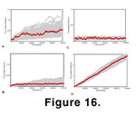 Directional, stabilizing, and randomly fluctuating selection each leave a distinctive imprint on the distribution of morphological distances, a phenomenon that is well known for univariate traits (e.g.,
Gingerich 1993;
Hansen and Martins 1996;
Roopnarine 2001;
Figure 16). The three modes influence the scaling relationship between short- and long-term evolutionary divergences in different ways, and the patterns can be used to infer the average evolutionary mode responsible for the differences among phenotypes.
Directional, stabilizing, and randomly fluctuating selection each leave a distinctive imprint on the distribution of morphological distances, a phenomenon that is well known for univariate traits (e.g.,
Gingerich 1993;
Hansen and Martins 1996;
Roopnarine 2001;
Figure 16). The three modes influence the scaling relationship between short- and long-term evolutionary divergences in different ways, and the patterns can be used to infer the average evolutionary mode responsible for the differences among phenotypes.
In directional selection, the rate of divergence over very short intervals is equal to very long intervals, and the morphological distance from the ancestor increases linearly with time. Morphological distance is a straight, diagonal line when plotted against time since divergence.
In randomly fluctuating selection, divergence from the ancestral form is greater over short intervals than over long ones, so that morphological distance increases curvilinearly with time. Drift leaves exactly the same imprint and randomly fluctuating selection, but the rate of divergence in the former is much slower. It is not correct that evolution in these modes "slows down"
(Kinnison and Hendry 2001;
Sheets and Mitchell
2001) – after all, we know that the rate of change at each generation remains the same on average throughout the simulation because the distribution of selection coefficients in the simulation is kept constant – but, rather, the probability that selection will take the shape at least some distance back towards its ancestral form increases with the amount of divergence
(Berg 1993;
Gingerich
1993). In other words, the chance increases with time that a long run of selection coefficients of the same sign will take the shape towards the ancestral form rather than away from it. The overall effect is that the net evolutionary divergence is greater over short intervals than long intervals, and the expectation of morphological distance is a function of the square root of the number of generations since common ancestry. Morphological distance forms a curved line when plotted against time since divergence.
In stabilizing selection, the first few thousand generations look like the randomly fluctuating pattern, but divergence then settles down to a roughly constant distance. Morphological distance is distributed as a straight, horizontal line when plotted against time since divergence. Note that with the parameters used here, the rate of evolution over short intervals is faster than over a similar interval under neutral drift, but total divergence is less over long intervals. Many tests of evolutionary mode are based on the assumption that neutral evolution is intermediate in rate between directional and stabilizing selection, regardless of the interval measured
(Turelli et al. 1988;
Lynch 1990;
Spicer
1993). The relation between the two modes will depend on the curvature of the stabilizing adaptive surface, as well as on the existence and magnitude of transient stochastic selection on the surface.
What Imprint Do Real Data Have?
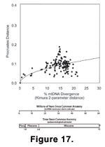 Morphological distances among real shrew
molars are distributed as though they evolved under randomly fluctuating selection
(Figure 17). In this graph, morphological distance in molar shape is plotted against mtDNA sequence divergence, which serves as a proxy – albeit an imperfect one – for time since common ancestry. Each point is a pairwise comparison between two taxa: some populations within the same species, some congeneric species, and others species belonging to different genera (see
Polly 2003a for more details). Morphological distance between the two is measured as Procrustes distance between the same nine landmarks used in the simulations. Phylogenetic divergence is measured as a Kimura 2-parameter distance in the cytochrome
b mtDNA sequences of the two taxa. This genetic distance is expressed as the percentage by which the two sequences differ, taking into account the probability of homoplasy at any position within the sequence. Generally, this measure of genetic difference increases linearly with time since common ancestry – though chance and homoplasy obscure this pattern – and so can be used as a coarse measure of time since common ancestry when direct palaeontological estimates are not available
(Brown et al. 1979;
Springer
1997). A second axis is shown with the genetic distances converted into millions of years using a rate of divergence of 2% per million years
(Brown et al. 1979;
Klicka and Zink 1997,
1998). Shrews are not well-studied palaeontologically, but coarse estimates of divergence times among the same taxa can be made from the fossil record (Repenning 1967;
Harris 1998;
Rzebik-Kowalska 1998;
Storch et al.
1998). This comparison suggests that molecular clock estimates may be overestimating divergence times, but in any event the last common ancestor of the most distantly related
Sorex taxa was at least 15 million years ago sometime during the Middle Miocene. The x-axis of the figure is thus 15 or more times longer than the simulations in
Figure 16.
Morphological distances among real shrew
molars are distributed as though they evolved under randomly fluctuating selection
(Figure 17). In this graph, morphological distance in molar shape is plotted against mtDNA sequence divergence, which serves as a proxy – albeit an imperfect one – for time since common ancestry. Each point is a pairwise comparison between two taxa: some populations within the same species, some congeneric species, and others species belonging to different genera (see
Polly 2003a for more details). Morphological distance between the two is measured as Procrustes distance between the same nine landmarks used in the simulations. Phylogenetic divergence is measured as a Kimura 2-parameter distance in the cytochrome
b mtDNA sequences of the two taxa. This genetic distance is expressed as the percentage by which the two sequences differ, taking into account the probability of homoplasy at any position within the sequence. Generally, this measure of genetic difference increases linearly with time since common ancestry – though chance and homoplasy obscure this pattern – and so can be used as a coarse measure of time since common ancestry when direct palaeontological estimates are not available
(Brown et al. 1979;
Springer
1997). A second axis is shown with the genetic distances converted into millions of years using a rate of divergence of 2% per million years
(Brown et al. 1979;
Klicka and Zink 1997,
1998). Shrews are not well-studied palaeontologically, but coarse estimates of divergence times among the same taxa can be made from the fossil record (Repenning 1967;
Harris 1998;
Rzebik-Kowalska 1998;
Storch et al.
1998). This comparison suggests that molecular clock estimates may be overestimating divergence times, but in any event the last common ancestor of the most distantly related
Sorex taxa was at least 15 million years ago sometime during the Middle Miocene. The x-axis of the figure is thus 15 or more times longer than the simulations in
Figure 16.
The real data have the same curvilinear pattern of morphological divergence found in randomly fluctuating selection and drift. The pattern is neither linear, like directional selection, nor flat like stabilizing selection. Furthermore, the rate of divergence is too high for drift, ruling out that mode as well. In the real data, divergences of one million years are roughly the same as 2-3% sequence divergence and have associated Procrustes distances of 0.05 to 0.75. Even in the less conservative drift simulation that used
Ne= 70, the largest Procrustes distances reached over 1,000,000 generations were less than 0.025. The real data have a much slower divergence than in the randomly fluctuating selection simulation, though, which reached morphological distances of 0.5 in only 1,000,000 generations, whereas the real data only have distances as high as 0.25 over 10 to 15 million years (generation lengths in shrews are roughly one year long). Clearly, the selections intensities driving molar shape evolution in shrews are lower than those measured in
Cantius.
A statistical test for mode could be developed from the curvatures and slopes of best fit lines through the Procrustes distributions generated by the simulations. Such a test is beyond the scope of the present paper, but visual inspection is enough to indicate that the curvature of the line through the real data is enough to rule out either directional or stabilizing selection, and the amount of shape divergence is too great for drift.
While impossible to test here, it can be hypothesized that the effects of mutation and selection on the interlocking between occluding teeth explain both the higher-than-neutral but still relatively slow rate of change. Shrew molars are of the tribosphenic type, and have a tight, complicated fit between their three-dimensional cusps, blades, and basins
(Butler 1961;
Evans and Sanson
2003). This lock-and-key mechanism ensures that occluding teeth must evolve together
(Polly et al.
2005). If a crown feature on one tooth changes, then functional selection will either remove that variant or favour a corresponding change on the counterpart tooth. Because of this
functional constraint, tooth morphology cannot be free to drift (presuming that occluding teeth are under somewhat independent genetic control), but selection may not be directional and will be slow because any change will require a corresponding one in another tooth. Ultimately, these functional constraints will impose morphological boundaries beyond which evolution cannot pass. Several of these simulations pass those boundaries, most notably directional selection, creating nonsense tooth shapes. If evolution were to approach those boundaries, stabilizing selection would prevent further change. The pattern of divergence among the real shrew taxa shows no sign that such boundaries are exerting an effect.
Phylogeny Reconstruction of Shape
An important feature common to all the evolutionary modes is that there is almost no chance that a derived morphology will be exactly like the ancestral one. In other words, the chance that homoplasy will recreate precisely the ancestral condition of a multivariate trait is nearly nil. This observation is important for phylogeny reconstruction, because it means that a predictable relationship exists between divergence in quantitative measures of multivariate morphology and time since common ancestry. In the directional selection, random selection and drift modes, a derived descendant morphology will be different from its ancestral condition and the amount of difference will have a linear relationship with the phylogenetic time elapsed. Multivariate quantitative phylogeny reconstruction algorithms are capable of recovering branching patterns when such conditions are obtained (Felsenstein
1988). Only in the case of strong stabilizing selection, in which morphology does not diverge from its ancestral form, is phylogeny not easily recoverable – even here, though, a problem with reconstructing phylogeny only arises when the boundaries of the stabilizing selection have been visited many times. For that period when lineages of a clade are wandering around the peak of an adaptive landscape without being driven back towards its centre, the pattern of divergence will be like that of fluctuating selection and phylogeny will be recoverable.
Univariate traits, such as trait size, do not have this expectation of divergence from the ancestral form. Regardless of the length of time, the most likely descendent value for a univariate trait is the same as its ancestor, even though the probability of a large difference increases with the number of generations. With univariate traits, the chance that homoplasy will recreate the precise ancestral condition is fairly high. The reason that multivariate traits, such as tooth shape, behave differently can be understood by thinking of them as a collection of several univariate traits: the probability that all of the traits will return to their ancestral values at the same time is small, even though each one has a high expectation of doing so; the more variables there are in the complex morphology, the less likely the chance that homoplasy will precisely recreate the ancestral form. (Incidentally, this observation explains the difference in rate scaling of univariate molar size
[Polly
2001b] as compared to multivariate molar shape [Polly
2002] in viverravid carnivorans.)
The potential of morphometric shape for phylogeny reconstruction can be seen in
Simulation 5
(Figure 15). The phenotypes within each clade share derived similarity not present in the ancestor or in the other. The red clade, for example, has a large, wide talonid basin at the posterior end of the tooth, while the blue clade has a short, narrow talonid. The shared derived similarity of each clade can be seen not only in the morphology itself, but also in the positions of the taxa within the principal components principal components space. In that space, any point away from the origin of the two axes represents a derived morphology, and the two red dots lie in a common derived space separate from where the two blue dots lie. The position of the taxa within PC space is the key to reconstructing phylogeny from morphometric representations of shape. Each axis of PC space can be treated as an independent trait, and the score of each taxon on that axis as its trait value; the combination of values on the different axes will be unique for each taxon, but related taxa will share similar derived values different from zero on many of the axes. To reconstruct phylogenetic relationships, one must find the tree that best explains the positions of the taxa simultaneously across all of the PC axes
(Polly 2003a,
b). When the traits have evolved under a Brownian motion mode of evolution, which appears to be the case for shrew molar teeth, then a maximum-likelihood method for continuous traits would be an appropriate algorithm
for phylogenetic analysis (Felsenstein 1973,
1981,
1988,
2002).
On "Morphological Clocks"
Complex morphology that evolves under randomly fluctuating selection, drift, or directional selection can be used as a coarse "morphological clock" in the same way
that molecular sequence divergence is used
(Polly
2001a). Because morphological distances increase in linear or curvilinear fashion under these modes of evolution, with them it is possible to predict the time since divergence of two taxa when one knows the Procrustes distance between their shapes and when one has an estimate of the per-generation rate of evolution. The principle is the same as with neutral molecular sequence divergence
(Kimura
1983), though the relationship between morphological shape to time is not as tightly linear.
The error in morphological clocks, especially under randomly fluctuating selection, would be large, however. For example, the best estimate of time since divergence for two taxa with a molar Procrustes distance of 0.25 would be 600,000 years given the parameters used in simulating randomly fluctuating selection
(Figure 16); however, divergences as small as 200,000 year can produce distances of 0.25, as can divergences well over 1,000,000 with the same parameters. The situation is better with directional selection, where a Procrustes distance of 1.0 implies a divergence time of about 375,000 years, with a range of possibilities from 220,000 to 400,000. In some cases, however, these estimates may be useful when no other data on divergence times are available. More often, though, direct stratigraphic estimates of common ancestry based on known
fossil occurrences of taxa will probably be better than such "morphological clock" estimates.
P-matrix Effects and Limitations
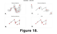 The P matrix influenced the distribution of phenotypes that could evolve; some morphologies were likely, and some nearly impossible. These constraints can easily be seen in the phenotypic space
(Figure 18). Each panel shows the 100 evolving phenotypes from the four main simulations. The effect of the correlations imposed by
P can be most readily seen in the results of randomly fluctuating evolution. The positions of each landmark are shown, and a 95% confidence ellipse has been drawn around them.
P prohibits, or at least renders improbable, those phenotypes that lie outside the trajectories of the expanding ellipses. Had there been no covariances among the landmarks, then the confidence ellipses would be perfectly circular and any phenotype would be possible given enough generations. The
P matrix used in these simulations was estimated from a real population, and so the constraints on morphological evolution imposed by it are probably real. The correlations recorded in
P come from many sources: developmental interactions, genetic pleiotropy, and chance sampling among them.
The P matrix influenced the distribution of phenotypes that could evolve; some morphologies were likely, and some nearly impossible. These constraints can easily be seen in the phenotypic space
(Figure 18). Each panel shows the 100 evolving phenotypes from the four main simulations. The effect of the correlations imposed by
P can be most readily seen in the results of randomly fluctuating evolution. The positions of each landmark are shown, and a 95% confidence ellipse has been drawn around them.
P prohibits, or at least renders improbable, those phenotypes that lie outside the trajectories of the expanding ellipses. Had there been no covariances among the landmarks, then the confidence ellipses would be perfectly circular and any phenotype would be possible given enough generations. The
P matrix used in these simulations was estimated from a real population, and so the constraints on morphological evolution imposed by it are probably real. The correlations recorded in
P come from many sources: developmental interactions, genetic pleiotropy, and chance sampling among them.
Limits exist to the amount of morphological evolution possible with a particular
P matrix. Its correlations impose limits to how much a particular part of the morphology can change and still be biologically compatible with the others. This phenomenon is most evident in the results of directional selection
(Figure 18B). The phenotypes move rapidly away from their ancestral form under directional selection, and after only 50,000 to 100,000 generations, landmarks have started to move into biologically incompatible positions. By 130,000 generations some points have fused, and by 170,000 begun to move past one another. From that point on, the simulated morphologies could not function as real teeth, demonstrating the limits that
P imposes on diversification. In life, three possibilities may exist: (1) evolution progresses slowly without reaching the limits of
P; (2) stabilizing selection prevents the phenotype from reaching those limits by pushing it back towards the ancestral form; or (3)
P itself changes to accommodate new, functionally viable morphologies that are radically different from the ancestral form.
But does P remain constant in real biological systems? One of the assumptions of the simulations was that
P did remain constant, but this issue is of major current concern in evolutionary genetics (Roff 1997;
Lynch and Walsh
1998). Logically, phenotypic and genetic covariances must evolve given enough time because if they did not, all organisms would have morphologies of roughly the same form (Lofsvold
1986). Genetic studies have demonstrated that showing that
P (and G, the heritable phenotypic variances and covariances) can change significantly, even among closely related species (Lofsvold
1986; Kohn and Atchley 1988;
Steppan 1997;
Badyaev and Hill 2000;
Roff et al.
2004). However, the changes in covariances, even when statistically significant, are often small, suggesting that trait correlations evolve slowly and remain broadly the same over long periods of phylogenetic divergence
(Kohn and Atchley 1988;
Brodie 1993;
Steppan 1997;
Arnold and Phillips 1999;
Roff et al.
2004). In shrew molars,
P has been demonstrated to evolve over timescales as short as 10,000 years, but the effect of those changes on the overall covariance structure is small
(Polly
2005). In principle, the simulation presented in this paper could be adapted to allow for a changing variance-covariance matrix.
