INTRODUCTION
Stochastic computer simulation is an important method
for comparing the evolutionary patterns and processes associated with radically
different intervals of time (Raup and Gould 1974;
Ibrahim et al.
1995).
Simulations allow the extrapolation of microevolutionary processes to
macroevolutionary timescales: populations can be evolved for millions of
generations using particular parameters (effective population sizes, phenotypic
variances, and heritabilities) and processes (directions and intensities of
selection, drift). The adequacy of population-level phenomena for explaining
macroevolutionary patterns can be tested by comparing the results with real
morphological diversity, or, conversely, population-level parameters can be
reverse engineered from comparative data by systematically varying the
parameters used in the simulations. Whereas simulations have been devised for
comparatively simple traitssuch as size, shell shape, or gene frequenciesa
procedure for modelling the long-term evolution of complicated morphologies
using quantitative genetic parameters remains difficult for most
palaeontological researchers.
This paper demonstrates how to perform a simulation of the evolution of almost any rigid morphological shape that can be represented geometrically (e.g., using landmarks or outlines in either two or three dimensions), regardless of its complexity. A crucial requirement is the availability of a sample from which population-level phenotypic covariances can be estimated. Directional, stabilizing, and random selection are simulated as walks in the empirical variation space defined by the principal components of the phenotypic covariance matrix. The morphological shape, or phenotype, at any step of the simulation can be retrieved, visualized, or utilized for quantitative comparisons. Simulations can be run multiple times for millions of generations to demonstrate the effects of microevolutionary processes over palaeontological timescales. The simulated morphologies can be used for statistical comparison with real comparative data from the fossil (or extant) record.
The simulation procedure is demonstrated by looking at the effects of directional selection, stabilizing selection, randomly fluctuating selection, and genetic drift on the long-term evolution of mammalian molar shape. Each of these evolutionary modes leaves a distinctive imprint on the distribution of morphological shape, a feature that can be used to estimate the mean mode that produced real morphological shapes in a particular lineage or clade. In this paper, I compare the outcomes of simulations of the evolution of molar crown shape in a single species of shrew,
Sorex araneus (Soricidae, Lipotyphla, Mammalia) to the real diversity of molar shape in species belonging to the same clade. A simulation of randomly fluctuating selection is also applied to a branching phylogeny in order to determine how derived morphometric shape accrues in independent
clades.
Sorex araneus, the Eurasian common shrew, is a
widespread and genetically interesting animal. Today, the species is spread over
most of Europe and across Siberia and Central Asia beyond Lake Baikal. It is
genetically subdivided into more than 70 named chromosomal races (Wójcik et al.
2003), and Quaternary fossil samples can be assigned to broad subgroups within
these races with reasonable accuracy (Polly
2003a).
S. araneus is part of a larger species complex that is peculiar in that
males typically have an extra X chromosome, in addition to the normal mammalian
complement of XY (Zima et al.
1998). In humans, this condition is
abnormal and referred to as Kleinfelter's syndrome. The
S. araneus complex evolved no more than 2.5 million years ago (Fumagalli
et al. 1999). Species within the group which include
S. coronatus, S. granarius, S. samniticus, S. arcticus,
and
S. tundrensis are often difficult to distinguish on non-morphometric
morphological grounds; hence, the fossil specimens have been usually referred to
S. araneus sensu lato. S. araneus and its relatives have a
rich fossil record covering three continents (Harris 1998;
Rzebik-Kowalska 1998;
Storch et al. 1998). The earliest probable member of the broader group
is from the Late Pliocene of Schernfeld, Germany (Dehm
1962), and by the
mid-Pleistocene they were widespread in Europe and Asia. In North America the
group was present in the form of
S. arcticus by the Late Pleistocene as far south as Arkansas and east as
West Virginia (Kurtén and Anderson 1980;
Semken 1984;
Harris
1998).
Typically the species
reproduces at a rate of one or two generations per year.
The Importance of Phenotypic
Covariances
 Empirically measured phenotypic covariances are an important part of this simulation procedure because they overcome a fundamental difficulty: morphological structures have patterns of correlation that channel their variation and evolution in non-random ways
(Olson and Miller 1958;
Zelditch et al.
1992). Parts of a biological structure do not vary randomly with respect to one another; rather, their topographical relationships are constrained by growth, genetics, function, materials, and general physical laws
(Maynard Smith et al. 1985;
Arnold
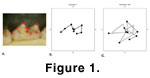
1992). Simulations that do not take into account these correlations quickly produce biologically unrealistic morphologies
(Figure 1).
Empirically measured phenotypic covariances are an important part of this simulation procedure because they overcome a fundamental difficulty: morphological structures have patterns of correlation that channel their variation and evolution in non-random ways
(Olson and Miller 1958;
Zelditch et al.
1992). Parts of a biological structure do not vary randomly with respect to one another; rather, their topographical relationships are constrained by growth, genetics, function, materials, and general physical laws
(Maynard Smith et al. 1985;
Arnold
1992). Simulations that do not take into account these correlations quickly produce biologically unrealistic morphologies
(Figure 1).
While it is difficult to link correlations to their various possible causes, it is relatively straightforward to measure their combined effects on a species or population. The phenotypic covariance matrix (P) describes the amount of variation (variances) in each part of a complex structure and the correlation (covariance) among the parts.
P provides information on the correlated response of parts of the structure relative to one another. Traits that are united by a particular constraint will have high covariances, while those that are unconstrained will have little or no covariance.
P can be measured from a sample of individuals randomly drawn from a population or species, such as the individuals found in many museum collections. The number required will depend on how extensive variation is in the particular structure being studied, but for vertebrate traits such as teeth and skulls a sample size of 10 can be minimally sufficient, although 20 to 50 individuals will yield a more accurate estimate.
The simulation procedure described in this paper is simplified by making use of the principal components of
P, rather than P itself. Every covariance matrix can be described as a series of principal components that represent independent components, or portions, of the variation and covariation in the original matrix. In technical terms, principal components are a series of orthogonal (or uncorrelated) axes known as
eigenvectors, each of which describes a particular amount of the total variance as indicated by the
eigenvalues (Blackith and Reyment 1971;
Tatsuoka and Lohnes
1988). The advantage to the principal components is that a univariate simulation can be run for each of the eigenvectors and the results summed over all
components to produce the full multivariate simulation
(Figure 2). 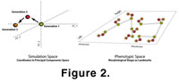 This shortcut is possible because the individual components are statistically independent of one another, and it greatly reduces the number of calculations that are required at each step of the simulation. When the simulations span hundreds of thousands or millions of steps, the savings are important. While the principal component space of the example is only shown in three dimensions, this procedure may be carried out across as many as applicable to a given dataset. In the simulations presented below, shape variation is evolved in 15 eigenvector dimensions.
The use of the principal components also overcomes a
difficulty associated with the fact that phenotypic covariance matrixes of
geometric shape are singular. Singular
P matrices result when some variables do not have any variation of their
own which is independent of the others. All geometric morphometric covariance
matrixes are singular because some of the biological variation size,
orientation, and position is removed from the data by superimposition (Gower 1975;
Rohlf and Slice 1990;
Rohlf
1999). A singular matrix can be
described by a set of principal components whose number is smaller than the
number of variables in the original
P matrix. This reduction in the number of variables also improves the
computational efficiency of the simulation. Principal components of a singular
matrix can be found using a standard procedure called Singular Value
Decomposition (Golub and Van Loan
1983).
Relation to Models of Multivariate
Evolution
Lande (1976,
1979) pioneered the study of the evolution of correlated characters. He provided equations for the response of phenotypes to selection and drift that were based on the concepts of adaptive landscapes first proposed by
Simpson (1944,
1953) and
Wright
(1968). He showed that the multivariate response to selection depends on the heritable, or additive genetic, covariances among the traits, as well as on the direction and magnitude of selection applied to each trait. Lande's multivariate approach has been widely used
in microevolutionary studies
(Lande 1986;
Lande and Arnold 1983;
Atchley and Hall 1991;
Cheverud 1995;
Marroig and Cheverud 2001;
Klingenberg and Leamy 2001;
Arnold et al.
2001), but seldom used to explore evolution over timescales as large as those in the fossil record (but see
Cheetham et al. 1993,
1994,
1995).
The simulation method described here is a modification of Lande's evolutionary model.
Lande (1979) described the evolution of multivariate morphology as
-
 (1)
(1)
where  is the change in the mean morphology of a population over the space of a single
generation,
G is the additive genetic covariance matrix, and
is the change in the mean morphology of a population over the space of a single
generation,
G is the additive genetic covariance matrix, and  is the series of selection coefficients that are applied to each variable used
to describe the morphological structure.
G represents that portion of P which is heritable, or passed,
from parents to their offspring.
is a set of selection coefficients (or drift
coefficients), one for each of the variables used to describe the phenotype. If
G is known and a particular set of is
applied to it, then the change in the mean phenotype for that generation is .
is the series of selection coefficients that are applied to each variable used
to describe the morphological structure.
G represents that portion of P which is heritable, or passed,
from parents to their offspring.
is a set of selection coefficients (or drift
coefficients), one for each of the variables used to describe the phenotype. If
G is known and a particular set of is
applied to it, then the change in the mean phenotype for that generation is .
Unfortunately, G is unknown for most morphological structures and for all palaeontological species. However, we can substitute
P for G by adding an extra parameter, heritability, to the simulation. The basic formula for morphological change at each generation in the simulations is, therefore,
-
 (2)
(2)
where is the
vector of selection coefficients, and
H is a heritability matrix that transforms P into G.
Because
H is also unknown, it must be simulated along with .
It is convenient to simulate
H as a single vector (H
is a vector the same length as ), rather
than as both a vector and a matrix because it reduces the number of computations
and because the elements of vector
H are equivalent to per-generation rates of
morphological change in standardized variance units, which are commonly reported
in palaeontological or comparative studies (Gingerich 1993;
Kingsolver et al.
2001).
This simulation thus does not represent a "constant heritability" model
(Lande 1976;
Spicer
1993) because
H forms part of the random parameter. It is also not a mutation-drift-equilibrium model
(Turelli et al. 1988;
Spicer
1993) because the phenotypic variance in each generation is held constant as part of
P. In nature, variance in a population is a balance between that which is removed by selection and that which is produced by mutation and recombination. In principle, a mutation-drift model could be simulated, but the parameter of the mutational variance would be difficult to estimate for shrew molars. In practice, the assumption of a stochastically constant variance is not unrealistic because the total variance in shrew molar shape does not change dramatically over long periods of evolutionary time
(Polly
2005).
Technical discussions of the effect of transforming P into its principal components and the effects of simulations on a singular
P matrix are found in the Appendix.
