RESULTS AND DISCUSSION

Principal Components

A principal components scatter of the fossil and recent calcanea is shown in Figure 4. The distribution of shapes was primarily functional, though low-level taxonomic relationships were also apparent in that the felids and mustelids each formed clusters. Higher level phylogenetic relationships were not reflected in the shape space distributions. Canis, for example, fell close to the felids, even though it is only distantly related, whereas Crocuta fell far from its kin the felids.

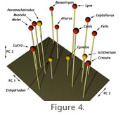
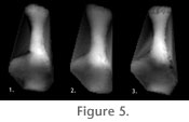
The first principal component, which explained 28.7% of the total variance in shape (Table 3), described differences in calcaneum shape associated with mobility at the lower ankle joint (LAJ) and stance. Plantigrade taxa with mobile LAJs like Bassaricyon and Ailurus fell at one end of PC 1 and digitigrade taxa with immobile LAJs like Crocuta, Felis, and Canis were at the opposite end. Calcanea with broad sustentacular facets positioned anterior to the calcaneoastragalar facet and broad distal regions with peroneal tubercle were found at the mobile end of the axis, whereas calcanea with proportionally smaller sustentacular facets positioned lateral to the calcaneoastragalar facet and a narrow, angled distal calcaneum were at its immobile end (Figure 5.1).

PC 2 explained 18.5% of the total variance (Table 3) and also described functional differences of the calcaneum. Calcanea with blocky distal ends, gently curved calcaneoastragalar facets, and thick calcaneal processes were at one end of the axis and bones with longer distal ends, sharply curved calcaneoastragalar facets, and narrow calcaneal processes were at the opposite end. These morphologies are associated with plantigrade and digitigrade postures, respectively.

PC 3 explained 13.9% of the total variance (Table 3). Overall breadth relative to length of the calcaneum was described by this axis, include correlation of the length of the sustentacular and peroneal processes. The mediolateral curvature of the calcaneoastragalar facet was also associated with this axis.

Locomotor Differences in Extant Taxa

Carnivores with four toes had, on average, narrower distal calcanea and broader sustentacular facets than did those with five toes (Figure 6.1). Plantigrade taxa had broader sustentacular facets placed more distally than did digitigrade taxa (Figure 6.2). The shape of the arboreal calcaneum was similar to the plantigrade one, and the average terrestrial calcaneum was similar to the digitigrade one (Figure 6.3). Scansorial and natatorial calanea both have distal ends that are angled medially on average, with a larger peroneal process on the natatorial one. Semifossorial calcanea have a straight distal end, but a large peroneal process. Additional functional differences have been discussed in Polly (2008).

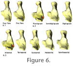
Locomotor Inference in Fossil Taxa

The four fossil calcanea were categorized for digit number, stance, and locomotor type by finding the closest match between their shape and the shapes shown in Figure 6 (Table 4). In total 12 categorizations were made, three for each of the four taxa. Of those, 10 were correct and two were incorrect (Table 5). The amphicyonid Cynelos was incorrectly categorized as being digitigrade when it was likely plantigrade or semidigitigrade, and the otter Enhydriodon was categorized as terrestrial when it was really natatorial. Cynelos was probably miscategorized because it has a more posteriorly positioned sustentacular facet than does the plantigrade average. The fit of Cynelos to the digitigrade category was only marginally better than to the semidigitigrade one (Procrustes distances 0.0083 and 0.0098, respectively). Enhydriodon was probably miscategorized because the distal end of the calcaneum is not as angled, and the peroneal process is not as large as in the modern otter.

Cluster analysis (the grouping of specimens based on a measure of distance, often a Euclidean distance like the Procrustes distance) and Discriminant Function Analysis (DFA) could be used in place of our Procrustes matching and probability calculation. We preferred to match each unknown specimen to the mean shapes in each category, which is basically finding the fossil's nearest neighbour in multivariate shape space, because clustering algorithms necessarily distort shape distances as a compromise in creating a tree topology (Sneath and Sokal 1973; Prager and Wilson 1978). The probability that all but two categorizations could have been correct by chance is real, but small. The probability that toe number could have been categorized correctly in all four taxa equals the probability of a correct assignment (50%) multiplied over the number of assignments made (4): 0.5⁴ = 0.0625. The probability that stance could have been categorized correctly in three taxa and wrongly in one is the probability of a correct assignment (33.3%) multiplied over the number of correct assignments (3) multiplied by the probability of one incorrect assignment (66.7%): 0.33³ * 0.67 = 0.025. And the probability that locomotor mode could have been categorized correctly in three taxa and wrong in one is the probability of a correct assignment (20%) multiplied over the number of correct assignments (3) multiplied by the probability of one incorrect assignment (80%): 0.2³ * 0.8 = 0.0064. The probability of obtaining only two incorrect results across the whole analysis is obtained by multiplying these three probabilities together: P = 0.0625 * 0.025 * 0.0064 = 9.8 x 10^-6.

The Eigensurface Method

The gridding algorithm used here is an improvement over the one described by Polly (2008), who fit a rectangular grid of points to the surface. The present algorithm produces analytical points that are spread more evenly across the surface than the earlier algorithm. The density of points across the surface determines how much each part of the morphology contributes to the analysis; high densities of points on particular parts cause those parts to be weighted more heavily in the analytical results. This approach differs, however, from that used by MacLeod (2008) to analyze bivalve shell shape using an algorithm to reduce 'edge effects,' whose approach reduces 'edge effects', and is especially useful when applying coarse grids to specimen surfaces.

The approach used here also differs from that used by Mitteröcker et al. (2005), who extended the use of sliding semi-landmarks to 3D surfaces of human skulls. Their approach used a skeleton of curves to represent the main 3D contours of an object. The curves were then fitted with sliding semi-landmarks positioned so as to minimize differences in shape among the objects (Bookstein 1997). The semi-landmark approach uses a much lower density of surface points than does ours, and so captures the general configuration of the object without capturing finer-scale details of the surface variation. Advantages of the semi-landmark approach compared to ours is that the semi-landmark method can be applied to topographically complicated structures (e.g., mammalian skulls); disadvantages compared to ours is that the semi-landmark method suffers even more greatly from variable densities of points, thus weighting some regions of the object more because regions with high point density contribute more variance to the overall shape than do those with lower point density.

Wiley et al. (2005) described a procedure for "evolutionary morphing" of primate skulls, which is similar to Mitteröcker et al.'s (2005) method in that it uses semi-landmarks to represent large patches of surface, but also used individual landmark points to represent parts of morphology that could easily be characterized that way. Wiley et al.'s analysis was carried out on the landmark and semi-landmark points, which were then used to "morph" entire scan data sets.

Three-dimensional surface shape has also been analyzed using spherical Fourier harmonic descriptors (SPHARM) of surface scan data (Styner et al. 2006; McPeek et al. 2008). Whereas the method of deriving shape coordinates from the x,y,z surface data is very different with Fourier harmonics, the subsequent methods for statistical analysis and shape visualization are similar to our method and the ones of Mitteröcker et al. (2005) and Wiley et al. (2005).