| |
THE MODEL AND EXPERIMENTAL SETUP
The Planet Simulator
In order to realise our sensitivity experiments, we use the
earth system model of intermediate complexity (EMIC) Planet Simulator (Fraedrich
et al. 2005a, b). The spectral
atmospheric general circulation model (AGCM) PUMA-2 is the core module of the
Planet Simulator. The model has a horizontal resolution of T21 (5.6° × 5.6°).
Five layers represent the vertical domain using terrain-following
sigma-coordinates. The atmosphere model is an advanced version (e.g.,
including moisture in the atmosphere) of the simple AGCM PUMA', the atmosphere
module now includes schemes for physical processes such as radiation transfer,
large-scale and convective precipitation, and cloud formation. The atmosphere
model is coupled to a slab ocean and a thermodynamic sea ice model, which
means that the ocean circulation is not calculated, but the heat exchange
between the atmosphere and ocean is represented as a thermodynamic system. The
slab ocean model uses a constant mixed layer depth of 50 m (see
Lunkeit et al. 2007 for technical
details). The sea ice model (based on
Semtner 1976) calculates the sea ice thickness from the thermodynamic
balance at the top and the bottom of the ice assuming a linear temperature
gradient. In order to realistically represent the heat transport in the ocean,
the models use a flux correction. It is also possible to simply force the
model prescribed climatological sea surface temperatures (SSTs) and sea ice.
The thermodynamic ocean and sea ice model produces a reasonable amount of sea
ice under present-day conditions (cf. sec. Results),
but it tends to overestimate the modern sea ice volume. It is known that the
conception of the sea ice model shows a good performance under conditions with
seasonal and thin ice (see Lunkeit et al.
2007 and references therein), but the performance for multiyear ice is
less. The Planet Simulator also includes a land surface module. Amongst
others, simple bucket models parameterize soil hydrology and vegetation. As
compared to highly complex general circulation models, the EMIC conception of
the Planet Simulator is relatively simple, but the model proved its
reliability (e.g., Fraedrich et al. 2005b;
Junge et al. 2004). For a more
complete description of the model, we refer to the documentation of the Planet
Simulator (Fraedrich et al. 2005a,
b). For this study, we use three
present-day experiments (Table 1).
They all use basically the same modern boundary conditions as the highly
complex AGCM ECHAM5 (e.g., Roeckner et al.
2003, 2006), but atmospheric CO2
is set to 280
ppm (pre-industrial), 360 ppm (normal), and, and 700 ppm (enhanced),
respectively. The experiments are referred to as CTRL-280, CTRL-360,
and CTRL-700 in the following.
The Boundary Conditions
 As
a reference base of our Miocene CO2-sensitivity experiments, we use
a Late Miocene (Tortonian, 11 to 7 Ma) model experiment. In the following,
this experiment is referred to as TORT-280. In principle, boundary
conditions of TORT-280 (Table 1) are
based on Late Miocene simulations with the highly complex AGCM ECHAM4 coupled
to a mixed-layer ocean model (Steppuhn et
al. 2006; Micheels et al. 2007).
The same Late Miocene model configuration as in the present study was used for
another Tortonian sensitivity experiment with the Planet Simulator (Micheels
et al. 2009). In the Miocene experiments, the solar luminosity and the
orbital parameters are the same as in the present-day simulations. Orbital
parameters triggered the Quaternary glacial-interglacial cycles (e.g.,
Petit et al. 1999), but for the
Tortonian we refer to a time span of about 4 million years integrating over
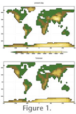
several orbital cycles. Due to the coarse model resolution, the Late Miocene
land-sea-distribution in TORT-280 is basically the modern one (Figure
1), but it includes the Paratethys (after
Popov et al. 2004). It is not possible
to resolve some differences between the present-day and Miocene continent
configurations. For instance, the present-day land-sea distribution represents
an open Central American Isthmus because the small modern land connection
between North and South America is lower than the model resolution. In the
Miocene, the Panama Strait was open (e.g.,
Collins et al. 1996) such as represented in our boundary conditions. The
palaeorography (Figure 1) is generally
lower than present in TORT-280 (Steppuhn
et al. 2006). For instance, the Tibetan Plateau reaches about half of its
present elevation. In fact, there is some debate about the palaeoelevation of
Tibet (e.g., Molnar 2005,
Spicer et al. 2003).
Spicer et al. (2003) suggest that
southern Tibet was at its present-day height over the last 15 Ma. However, the
mean elevation of the Tibetan Plateau in the Late Miocene was
lower-than-present (Molnar et al. 2005),
which is represented in our model configuration (Figure
1). As
a reference base of our Miocene CO2-sensitivity experiments, we use
a Late Miocene (Tortonian, 11 to 7 Ma) model experiment. In the following,
this experiment is referred to as TORT-280. In principle, boundary
conditions of TORT-280 (Table 1) are
based on Late Miocene simulations with the highly complex AGCM ECHAM4 coupled
to a mixed-layer ocean model (Steppuhn et
al. 2006; Micheels et al. 2007).
The same Late Miocene model configuration as in the present study was used for
another Tortonian sensitivity experiment with the Planet Simulator (Micheels
et al. 2009). In the Miocene experiments, the solar luminosity and the
orbital parameters are the same as in the present-day simulations. Orbital
parameters triggered the Quaternary glacial-interglacial cycles (e.g.,
Petit et al. 1999), but for the
Tortonian we refer to a time span of about 4 million years integrating over
several orbital cycles. Due to the coarse model resolution, the Late Miocene
land-sea-distribution in TORT-280 is basically the modern one (Figure
1), but it includes the Paratethys (after
Popov et al. 2004). It is not possible
to resolve some differences between the present-day and Miocene continent
configurations. For instance, the present-day land-sea distribution represents
an open Central American Isthmus because the small modern land connection
between North and South America is lower than the model resolution. In the
Miocene, the Panama Strait was open (e.g.,
Collins et al. 1996) such as represented in our boundary conditions. The
palaeorography (Figure 1) is generally
lower than present in TORT-280 (Steppuhn
et al. 2006). For instance, the Tibetan Plateau reaches about half of its
present elevation. In fact, there is some debate about the palaeoelevation of
Tibet (e.g., Molnar 2005,
Spicer et al. 2003).
Spicer et al. (2003) suggest that
southern Tibet was at its present-day height over the last 15 Ma. However, the
mean elevation of the Tibetan Plateau in the Late Miocene was
lower-than-present (Molnar et al. 2005),
which is represented in our model configuration (Figure
1).
 Another
important characteristic in our Miocene configuration is that Greenland is
lower as compared to today (Figure 1)
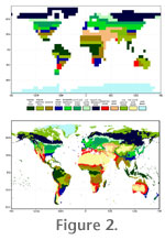
because of the absence of glaciers (Figure 2). Also
the palaeovegetation (Figure 2) refers to the
Tortonian (Micheels et al. 2007). In
particular, boreal forests extend far towards northern high latitudes, whereas
deserts/semi-deserts and grasslands are reduced as compared to the present. We
removed the modern Greenland glaciers (cf. above), and vegetation cover of the
Miocene runs refers to boreal forests. Instead of the present-day Sahara
desert, North Africa is covered by grassland to savannah vegetation in the
Tortonian experiments. Another
important characteristic in our Miocene configuration is that Greenland is
lower as compared to today (Figure 1)
because of the absence of glaciers (Figure 2). Also
the palaeovegetation (Figure 2) refers to the
Tortonian (Micheels et al. 2007). In
particular, boreal forests extend far towards northern high latitudes, whereas
deserts/semi-deserts and grasslands are reduced as compared to the present. We
removed the modern Greenland glaciers (cf. above), and vegetation cover of the
Miocene runs refers to boreal forests. Instead of the present-day Sahara
desert, North Africa is covered by grassland to savannah vegetation in the
Tortonian experiments.
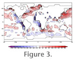
The ocean is initialised using 'palaeo-SSTs' from a previous
Tortonian run (Micheels et al. 2007),
and the Northern Hemisphere's sea ice is initially removed. After the
initialization, we continue the model integration using the slab ocean with
the present-day flux correction (Figure 3).
It is commonly known that because of the open Central American Isthmus the
northward ocean heat transport in the Miocene was relatively weak as compared
to today (e.g., Bice et al. 2000;
Steppuhn et al. 2006;
Micheels et al. 2007). Later on in the
Pliocene, the northward ocean heat transport
 was
stronger than today (e.g., Haywood et al.
2000a, b). It is not an easy task
to properly specify the ocean flux correction for a past climate situation (Steppuhn
et al. 2006). With additional sensitivity experiments, it would have been
possible to include different scenarios for the ocean heat transport. This is,
however, beyond the scope of the present study because we aim to analyse a
single factor, which is CO2. Therefore, we have chosen the modern
flux correction as an approximation for an intermediate state in between the
relatively weak Miocene and the relatively strong Pliocene ocean heat
transport. A recently published study (Tong
et al. 2009) focussed on CO2 in the Mid-Miocene using an AGCM
coupled to a slab ocean model. Therein, the setup of the slab ocean model,
i.e. the generation of the flux correction, is also based on present-day SSTs
and sea ice cover. was
stronger than today (e.g., Haywood et al.
2000a, b). It is not an easy task
to properly specify the ocean flux correction for a past climate situation (Steppuhn
et al. 2006). With additional sensitivity experiments, it would have been
possible to include different scenarios for the ocean heat transport. This is,
however, beyond the scope of the present study because we aim to analyse a
single factor, which is CO2. Therefore, we have chosen the modern
flux correction as an approximation for an intermediate state in between the
relatively weak Miocene and the relatively strong Pliocene ocean heat
transport. A recently published study (Tong
et al. 2009) focussed on CO2 in the Mid-Miocene using an AGCM
coupled to a slab ocean model. Therein, the setup of the slab ocean model,
i.e. the generation of the flux correction, is also based on present-day SSTs
and sea ice cover.
The CO2-Sensitivity Scenarios
The concentration of atmospheric carbon dioxide in the Miocene
is still debated and values vary from as low as 280 ppm (e.g.,
Pagani et al. 2005) to as high as 1000
ppm (Retallack 2001). As for the
pre-industrial control experiment CTRL, atmospheric CO2 is set to
280 ppm in the Tortonian reference simulation TORT-280. In addition, we run
six experiments for which we set pCO2 to 200, 360, 460, 560, 630, and
700 ppm (Table 1). These runs are
referred to as TORT-360 to TORT-700. All model experiments
except TORT-200 are integrated over 200 years. The equilibrium is achieved
after much less than 100 years. The last 10 years of each experiment are
considered for further analysis. TORT-200 is integrated over 100 years and it
is used to define a transitional experiment. From years 101 to 2100, the
atmospheric CO2 steadily increases by +1 ppm per year. This
experiment is named TORT-INC and covers the range of pCO2 from
200 ppm to 2200 ppm. The maximum of 2200 ppm corresponds to a value, which was
realised rather in the Eocene than later on (Pagani
et al. 2005). We do not design a specific experiment for 1000 ppm (Retallack
2001) because, on the one hand, this value as compared to other studies
(e.g., Cerling 1991;
MacFadden 2005;
Pagani et al. 2005) appears to be
rather high for the Miocene. On the other hand, it is already included in
TORT-INC except that the model might not be fully in equilibrium. For TORT-INC
at 1000, 1500, and 2000 ppm (i.e., in years 900, 1400, and 1900), we refer to
TORT-1500, TORT-1500, and TORT-2000, respectively. The
setup of all our experiments is summarised in
Table 1. |