| |
RESULTS
Global Averages of Temperature and Sea Ice Cover
 Figure
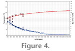
4 illustrates that in the Miocene and present-day simulations, the global
temperature increases and the global sea ice cover decreases with an increased
atmospheric carbon dioxide. The global temperature of the Tortonian runs is
generally higher than in the present-day simulations (if CO2 is the
same in CTRL and TORT). Accordingly, the sea ice cover of TORT-200 to TORT-INC
is also lower than in CTRL-280 to CTRL-700. With increasing CO2,
the global temperature and sea ice cover of TORT-INC follows quite well the
distribution of the other runs TORT-200 to TORT-700. Hence, the CO2
increase of +1 ppm is small enough to keep TORT-INC close to the equilibriums
of TORT-200 to TORT-700. Figure
4 illustrates that in the Miocene and present-day simulations, the global
temperature increases and the global sea ice cover decreases with an increased
atmospheric carbon dioxide. The global temperature of the Tortonian runs is
generally higher than in the present-day simulations (if CO2 is the
same in CTRL and TORT). Accordingly, the sea ice cover of TORT-200 to TORT-INC
is also lower than in CTRL-280 to CTRL-700. With increasing CO2,
the global temperature and sea ice cover of TORT-INC follows quite well the
distribution of the other runs TORT-200 to TORT-700. Hence, the CO2
increase of +1 ppm is small enough to keep TORT-INC close to the equilibriums
of TORT-200 to TORT-700.
Comparing CTRL-360 and CTRL-700 vs. CTRL-280 and the Tortonian
runs, the response on an increased pCO2 is more pronounced
in the present-day simulations. The temperature difference between CTRL-700
and CTRL-360 is +2.5°C, whereas it is +1.9°C between TORT-700 and TORT-360.
Sea ice cover is reduced by 2.9% (CTRL-700 minus CTRL-360) and by 2.1%
(TORT-700 minus TORT-360), respectively. Hence, the weaker response to a CO2
increase is explained by the generally lower amount of sea ice in the Miocene
experiments, i.e., the ice-albedo feedback is weaker.
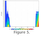 Figure
5 illustrates the zonal average sea ice cover of TORT-INC with respect to
CO2. A critical threshold for the Arctic ice cover is around 1,250
ppm. At this level, the northern sea ice entirely vanishes for the first time,
but it sensitively responds on climate fluctuations. If there is a small
deviation (climate variability), ice-free conditions cannot be maintained.
With an atmospheric carbon dioxide concentration of about 1,400 ppm, the
Northern Hemisphere is permanently ice-free in TORT-INC. The sea ice cover on
the Southern Hemisphere is generally maintained. However, only a few small
fractions of sea ice remain if pCO2 is higher than about
1,500 ppm. Figure
5 illustrates the zonal average sea ice cover of TORT-INC with respect to
CO2. A critical threshold for the Arctic ice cover is around 1,250
ppm. At this level, the northern sea ice entirely vanishes for the first time,
but it sensitively responds on climate fluctuations. If there is a small
deviation (climate variability), ice-free conditions cannot be maintained.
With an atmospheric carbon dioxide concentration of about 1,400 ppm, the
Northern Hemisphere is permanently ice-free in TORT-INC. The sea ice cover on
the Southern Hemisphere is generally maintained. However, only a few small
fractions of sea ice remain if pCO2 is higher than about
1,500 ppm.
Zonal Average Temperatures
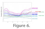 Figure
6 shows the zonal average temperatures of the simulations wherein the
Miocene experiments are represented against TORT-280 and the present-day runs
and TORT-280 against CTRL-280, respectively. TORT-280 is much warmer than
CTRL-280 at around 30°N (+4°C) and farther to the northern high latitudes
(+5°C). Close to the equator, CTRL-280 and TORT-280 do not differ much (less
than +1°C). Thus, TORT-280 represents a weaker-than-present meridional
temperature gradient of 4°C. The meridional gradient in TORT-200 is less
pronounced than in TORT-280, but it is still weaker than in CTRL-280. With
increasing carbon dioxide in the atmosphere, the low to high latitudes get
successively warmer, but polar warming is much more intense. In TORT-INC at
2,000 ppm, the high latitudes heat up by +9°C as compared to TORT-280, and
tropical latitudes are +3.5°C warmer. Thus, the temperature difference between
pole and equator is 5.5°C lower than in TORT-280. The successive reduction of
the meridional temperature gradient is a result of the sea ice-albedo feedback
(cf. Figure 4 and
Figure 5). The temperature difference
between TORT-2000 (i.e., TORT-INC at 2000 ppm) and TORT-1500 is generally less
than for TORT-1500 vs. TORT-1000. The weaker response is due to the fact that
northern sea ice vanishes at around 1,400 ppm (Figure
5). Figure
6 shows the zonal average temperatures of the simulations wherein the
Miocene experiments are represented against TORT-280 and the present-day runs
and TORT-280 against CTRL-280, respectively. TORT-280 is much warmer than
CTRL-280 at around 30°N (+4°C) and farther to the northern high latitudes
(+5°C). Close to the equator, CTRL-280 and TORT-280 do not differ much (less
than +1°C). Thus, TORT-280 represents a weaker-than-present meridional
temperature gradient of 4°C. The meridional gradient in TORT-200 is less
pronounced than in TORT-280, but it is still weaker than in CTRL-280. With
increasing carbon dioxide in the atmosphere, the low to high latitudes get
successively warmer, but polar warming is much more intense. In TORT-INC at
2,000 ppm, the high latitudes heat up by +9°C as compared to TORT-280, and
tropical latitudes are +3.5°C warmer. Thus, the temperature difference between
pole and equator is 5.5°C lower than in TORT-280. The successive reduction of
the meridional temperature gradient is a result of the sea ice-albedo feedback
(cf. Figure 4 and
Figure 5). The temperature difference
between TORT-2000 (i.e., TORT-INC at 2000 ppm) and TORT-1500 is generally less
than for TORT-1500 vs. TORT-1000. The weaker response is due to the fact that
northern sea ice vanishes at around 1,400 ppm (Figure
5).
Between CTRL-360 and CTRL-280, there are just minor
differences of less than +1°C, which is similarly seen from TORT-360 as
compared to TORT-280. However, CTRL-700 vs. CTRL-280 as compared to CTRL-360
vs. CTRL-280 demonstrates a more amplified polar warming than TORT-700 and
TORT-360 vs. TORT-280, respectively. The CO2 doubling from 360 ppm
to 700 ppm leads to a polar warming of +4°C under present-day conditions,
whereas it is only +3°C in the Miocene. In lower latitudes, the response to
the CO2 increase is about the same. Thus, the sea ice-albedo
feedback tends to be weaker under Miocene boundary conditions than using
present-day conditions (cf. Figure 4).
Spatial Temperature Anomalies
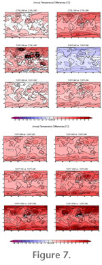 The
spatial distribution of mean annual temperature differences and the sea ice
margin between our simulations are shown in
Figure 7. The increase of CO2
leads to a generally more pronounced warming in the present-day experiments as
compared to the Miocene runs (_blank). For CTRL-280 to CTRL-700, the ice
volume is greater than in TORT-200 to TORT-2000 (cf. sec. 3.1 and 3.2).
Therefore, the ice-albedo feedback is more intense under present-day
conditions. Moreover, the Paratethys dampens the general warming trend due to
enhanced CO2 in the Miocene simulations. In TORT-200 as compared to
TORT-280, the cooling because of a decreased CO2 occurs primarily
in higher latitudes. This is a contrast to the other Tortonian runs.
Generally, interior parts of the continents become warmer when CO2
increases. Not until a high concentration of CO2 and ice-free
conditions are reached, polar warming is in the same order of magnitude as
over the continental areas. In Central Africa, temperatures in the Tortonian
runs remain more or less the same when increasing CO2. An
intensified evapotranspiration (evaporative cooling) dampens the temperature
increase due to the greenhouse effect. The
spatial distribution of mean annual temperature differences and the sea ice
margin between our simulations are shown in
Figure 7. The increase of CO2
leads to a generally more pronounced warming in the present-day experiments as
compared to the Miocene runs (_blank). For CTRL-280 to CTRL-700, the ice
volume is greater than in TORT-200 to TORT-2000 (cf. sec. 3.1 and 3.2).
Therefore, the ice-albedo feedback is more intense under present-day
conditions. Moreover, the Paratethys dampens the general warming trend due to
enhanced CO2 in the Miocene simulations. In TORT-200 as compared to
TORT-280, the cooling because of a decreased CO2 occurs primarily
in higher latitudes. This is a contrast to the other Tortonian runs.
Generally, interior parts of the continents become warmer when CO2
increases. Not until a high concentration of CO2 and ice-free
conditions are reached, polar warming is in the same order of magnitude as
over the continental areas. In Central Africa, temperatures in the Tortonian
runs remain more or less the same when increasing CO2. An
intensified evapotranspiration (evaporative cooling) dampens the temperature
increase due to the greenhouse effect.
The Sensitivity Experiments vs. Quantitative Terrestrial Proxy Data
Steppuhn et al. (2007)
established a method to compare Late Miocene model experiments with
quantitative terrestrial proxy data. We now use basically the same method to
test how consistent the mean annual temperatures (MAT) of the different Late
Miocene CO2 scenarios are as compared to the fossil record. The
main data set of terrestrial proxy data is given in
Steppuhn et al. (2007). All data for
mean annual temperature (MAT) are based on quantitative climate analyses of
fossil plant remains from the Tortonian stage (early Late Miocene, ~ 11 to 7
Ma). For most of the data, the Coexistence Approach (Mosbrugger
and Utescher 1997) was applied on micro- (pollen and spores) and
macro-botanical (leaves, fruits, and seeds) fossils. The results of this
method are 'coexistence intervals,' which express the minimum-maximum range of
temperature at which a maximum number of taxa of a given flora can exist.
Relying mainly on one reconstruction method reduces the impact of
methodological inconsistencies. However, such data are not yet available for
North America. Therefore, we also included some published quantitative climate
data based on the CLAMP technique (Wolfe
1993), which has proven to be a reliable method especially for climate
quantification on the American continent (cf.
Wolfe 1995,
1999).
 Because
such data usually do not include a minimum-maximum range of temperature, a
standard range of uncertainty of ±1 °C was assumed for the
data-model-comparison. We completed the
Steppuhn et al. (2007) data set with additional climate information from
Wolfe et al. (1997) and new data from the NECLIME program (see
http://www.neclime.de) published in
Akgün et al. (2007),
Bruch et al. (2007) and
Utescher et al. (2007). The actual
data set used in this study now comprises 78 localities. Because most of the
proxy data represent a climatic range from a minimum to a maximum mean annual
temperature at a locality, Steppuhn et al.
(2007) constructed a similar MAT range from the minimum and maximum mean
annual temperature of their 10-year-model integrations at the specific grid
points. In case of an overlap of both climate intervals, model results and
proxy data are defined to be consistent (i.e., the temperature difference is
equal zero); in case both intervals do not overlap, the smallest distance
between them is defined to be a measure for the inconsistency. We slightly
modify the validation method of Steppuhn
et al. (2007) because results of TORT-1000, TORT-1500, and TORT-2000 do
not represent a time series over 10 years. Instead of creating temperature
intervals from our simulations, we use "point" data. For TORT-1000 to
TORT-2000, the point data are simply the mean annual temperatures of the years
900, 1400, and 1900, respectively. For TORT-200 to TORT-700, the point data
are the mean annual temperatures averaged over the last 10 years of the model
integrations. Except of this difference, the validation method follows the
same principle as before (Steppuhn et al.
2007). Table 2 summarises the
overall agreement of the Tortonian simulations with proxy data. In
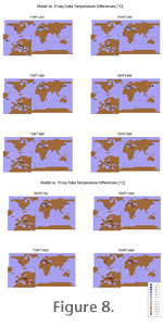
Figure 8, the temperature differences
between the simulations and proxy data are mapped for all localities. Because
such data usually do not include a minimum-maximum range of temperature, a
standard range of uncertainty of ±1 °C was assumed for the
data-model-comparison. We completed the
Steppuhn et al. (2007) data set with additional climate information from
Wolfe et al. (1997) and new data from the NECLIME program (see
http://www.neclime.de) published in
Akgün et al. (2007),
Bruch et al. (2007) and
Utescher et al. (2007). The actual
data set used in this study now comprises 78 localities. Because most of the
proxy data represent a climatic range from a minimum to a maximum mean annual
temperature at a locality, Steppuhn et al.
(2007) constructed a similar MAT range from the minimum and maximum mean
annual temperature of their 10-year-model integrations at the specific grid
points. In case of an overlap of both climate intervals, model results and
proxy data are defined to be consistent (i.e., the temperature difference is
equal zero); in case both intervals do not overlap, the smallest distance
between them is defined to be a measure for the inconsistency. We slightly
modify the validation method of Steppuhn
et al. (2007) because results of TORT-1000, TORT-1500, and TORT-2000 do
not represent a time series over 10 years. Instead of creating temperature
intervals from our simulations, we use "point" data. For TORT-1000 to
TORT-2000, the point data are simply the mean annual temperatures of the years
900, 1400, and 1900, respectively. For TORT-200 to TORT-700, the point data
are the mean annual temperatures averaged over the last 10 years of the model
integrations. Except of this difference, the validation method follows the
same principle as before (Steppuhn et al.
2007). Table 2 summarises the
overall agreement of the Tortonian simulations with proxy data. In
Figure 8, the temperature differences
between the simulations and proxy data are mapped for all localities.
On the global scale (Table
2), the experiment TORT-280 fits best with terrestrial proxy data, but
also TORT-200, TORT-360, and TORT-460 give more or less consistent results.
Discrepancies of TORT-200 to TORT-460 are within ±1°C. These deviations to the
fossil record are quite acceptable. As one might expect, TORT-2000
demonstrates the worst overall consistency to proxy data and is globally much
too warm.
Figure 8 shows details
of the comparison of model results and proxy data. TORT-200 and TORT-280
globally demonstrate the best agreement to proxy data, but they are
systematically too cool in higher latitudes. TORT-360 and TORT-460 indicate a
better agreement in higher latitudes. However, both runs tend to be slightly
too warm in the mid-latitudes, particularly in Europe. At the expense of
heating up lower and mid-latitudes, TORT-560 to TORT-2000 are continuously
more consistent to high-latitude proxy data.
Figure 8 illustrates that TORT-360 to
TORT-560 basically agree best with proxy data. This agreement seems to be in
contrast to Table 2, but one has to
keep in mind that the spatial distribution of proxy data is highly
concentrated on Europe. Consequently, discrepancies in this region are
over-weighted as compared to others. Our results support that pCO2
in the Late Miocene is within the range of 360 to 560 ppm. |