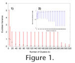
METHODS

In this section we describe the data used and our methods for determining diversities. We also describe our methods for additional tests using subsampling (rarefaction) and simulated habitat types. Extant communities can have spatially open configurations in which the inhabitants of one community can extend into neighboring communities (Whittaker 1972). To avoid confounding the analysis with such extant communities and to examine long-term relationships between biodiversity and tectonism, diversity measures are expressed per grid cell assemblage of fossils. We define an assemblage grid cell as the collection of marine fossil occurrences per 10,000 km. We calculated this by first computing the diversity measures for each grid cell (1° longitude x 1° latitude) and then scaling to a standard grid cell surface area assuming a spherical Earth. Each non-empty grid cell contained one or more co-occurring fossil observations, which contributed to its alpha and beta diversity. As in extant ecosystems, grid cells may consist of multiple habitat types, within which many of the activities of these marine populations occurred. In the absence of ecological observations, the lithological annotations of each fossil occurrence were used to simulate and assign each to a habitat type using a multivariate statistical clustering method. Source pool diversity and connectivity were also calculated for the neighborhood of each grid cell. Statistical properties of these indexes were analyzed regionally and through time.

Paleobiology Database

Our data were derived from the Paleobiology Database (PD 2008), one of the most extensively annotated compilations of fossil occurrences to date (Alroy et al. 2008). We focused our analysis on the most recent 57 m.y. of these data, which contain many of the best preserved and most detailed specimens of the fossil record. These 83,213 occurrences represent 8,821 published articles and include 25,595 species (5,773 genera) and 40 phylogenetic classes of marine fossil organisms. Of the 77,820 phylogenetically annotated occurrences (23,330 species), 62,689 (81%) occurrences or 17,446 (75%) of the species belong to the phylogenetic classes Bivalvia or Gastropoda (Table 1) indicating that mollusks are particularly well represented in the PD (Crame 2009).

Each occurrence downloaded from the PD is annotated with an environment of deposition and several fields describing lithology. We converted these observations from categories to numerical values using the PD's data entry criteria (PD 2008). For example, the depositional environment "foreshore" in the PD is reserved for occurrences with reported lithologies that are indicative of the intertidal zone between high and low tide. The mean of that range (zero) was taken to be the water depth for such an observation, as it was either submerged or emergent depending on the tide. Thus, for each of the 421 environmental and lithological combinations in our downloaded data, we have designated values for water depth and the percentage of sand, silt, clay, and lime mud (see Appendix Table 1). The subsequent scalar values for depth, sand, silt, clay, and lime mud were used as environmental characteristics to define the hyperspace volume for each habitat type within its landscape using cluster analysis.

Habitat Type Determination

In order to simplify exposition and computations of the data, a multivariate statistical cluster analysis technique, based on the k-means procedure of Hartigan (1975), was employed to identify unique habitat types, following the method used for ecoregionalization by Hargrove and Hoffman (2004). An improved version of a parallel clustering algorithm, developed by Hoffman and Hargrove (1999), was run on a high performance cluster computer. The clustering procedure consists of two parts: initial centroid or seed determination and iterative clustering of observations (fossil occurrences) until convergence is reached. Initial centroids (seeds), one for each of the k clusters, were selected at random from the fossil occurrence data. In the iterative clustering algorithm, fossil occurrence records are assigned to the nearest centroid, by Euclidean distance, in the m-dimensional phase space formed from the m environmental characteristics included in the analysis. Once all records are assigned to a centroid, the centroid locations in this phase space are recomputed as the mean of the observations assigned to that centroid. This process repeats until only a small number of observations are assigned to a different cluster between iterations. For this study, the convergence criteria was 0.5% of the n fossil occurrence records.

Since the number of clusters, k, is chosen a priori by the user, a series of clustering trials, with k = 5,10,20,40,60,...,320, were performed to determine a reasonable level of division for the data. Figure 1 shows a scree plot of the mean Euclidean variance for clusters at different levels of division. Around k = 40 this mean variance is reasonably small while the number of clusters is not too large to analyze. Therefore, the results presented here will be primarily for k = 40. Because clustering results can also be somewhat sensitive to the selection of initial centroids (seeds), a number of clustering trials were performed with different random seeds. Statistical correlations were consistent across the trials, so the results presented are not sensitive to the starting seeds. Table 2 shows example results of the clustering procedure.

Alpha and Beta Diversity

We used two primary measures of biodiversity: alpha diversity, the latitudinally scaled diversity of fossil species (or genera) within one grid cell, and Whittaker's beta diversity, the species or generic difference between two grid cells (Whittaker 1972). Beta diversity is calculated as D_c/D_b – 1, where D_c is the total diversity of species (or genera) in the composite of two grid cells, and Db is the mean diversity of species (or genera) from both grid cells. Empty grid cells, those without fossil occurrences, were excluded. For any grid cell assemblage, Ai, that touched only one occupied neighboring grid cell, N = 1, the calculation of beta diversity was exactly as described above. For any Ai where 2≤N≤8, beta diversity was calculated as the mean of all betas in the neighborhood (see Appendix Table 3). To complete the neighborhood for grid cells located at geographical edges (e.g., longitude 179°W to 180°W), we wrapped these neighborhoods to include grid cells at the opposite geographic extreme (e.g., longitude179°E to 180°E). No occupied grid cells in our data set appeared at latitudes above 89° north or south, therefore it was not necessary to wrap over the poles.

Source Pool Diversity and Connectivity

For the neighborhood of each grid cell we measured two additional indexes that describe the spatial continuity of these fossil data: source pool diversity and connectivity. Source pool diversity is equivalent to the total alpha diversity of the neighborhood excluding the grid cell of interest. Connectivity is the proportion of occupied adjacent grid cells. We express this as a ratio between 0 and 1, with 1 being a neighborhood in which each of the 8 neighboring grid cells is occupied by at least one fossil observation.

Subsampling Routine (rarefaction)

To test whether or not the correlations between diversity measures and simulated paleoecosystem factors could be the result of biased sampling intensity, assuming that the abundance of occurrences reflects sampling intensity, we computed diversity D from the complete list of fossil occurrences LI, and from the mean of 100 rarefied lists Li. For rarefied lists we randomly selected 100 fossil occurrences from each grid cell's fossil occurrence list using a uniformly distributed pseudo-random number generator (Park and Miller 1988). Each rarefied occurrence list represents a random subsample of its original list. Thus the rarefied diversity Di of a grid cell assemblage Ai is computed as the sum of unique genus (G, or species names S) drawn from Li, where Li is a random subsample of LI. In computing Li for each region in each sub-epoch in Table 3 we instead used occurrence lists of length 15 rather than 100 in order to consistently include Japan, which generally had occurrence lists shorter than 100.