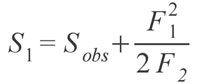
NON-PARAMETRIC SPECIES ESTIMATORS AND RAREFACTION

An obvious problem in palaeontology is the incompleteness of the record, and therefore our incomplete knowledge of the number of species present, whether locally or globally. Modern ecologists suffer from the same problem, whereby it is impractical to sample every single member of even relatively small communities of organisms (Chazdon et al. 1998). However, smaller samples still contain important information about the community and can be extrapolated from to provide estimates of the true richness of the total community. Of course, such extrapolations must account for sampling intensity and area (Gleason 1922; Preston 1948).

One of the most commonly used methods for dealing with unequal sampling intensity is rarefaction, or interpolation of the data (Sanders 1968). Rarefaction provides a method of comparison between different communities, whereby each community is "rarefied" back to an equal number of sampled specimens (Heck et al. 1975; Foote 1992; Colwell and Coddington 1994). Within the fossil package is a method for rarefaction known as a Coleman Curve (Coleman 1981; Coleman et al. 1982). This type of rarefaction is carried out through a resampling method rather than a rarefaction formula; resampling is computationally much simpler and faster, and provides indistinguishable results from the formula based method (Coleman 1981; Coleman et al. 1982; Colwell and Coddington 1994; Magurran 2004). The Coleman Curve is an empirical measure of the rarefied number of individuals, while the rarefaction function is a theoretical model of what the empirical curve would look like. Although rarefaction can be useful, it is very sensitive to the underlying pattern of species abundance, such that collections with much lower species evenness will often give lower estimates of species diversity than those with very even abundances, regardless if species diversities in reality are equal (See Gotelli and Colwell [2001] for an in-depth treatment of the issue.).

Although rarefaction interpolates data back, non-parametric species estimators extrapolate from the data to find what the 'true' number of species may have been (Colwell and Coddington 1994). The typical way these estimators operate is by using the number of rare species that are found in a sample as a way of calculating how likely it is there are more undiscovered species. As an example, the Chao 1 estimator (Chao 1984; Colwell and Coddington 1994) calculates the estimated true species diversity of a sample by the equation:

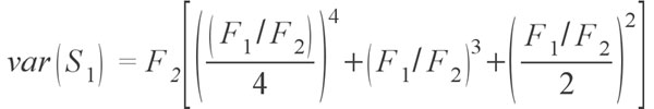
where Sobs is the number of species in the sample, F1 is the number of singletons (i.e., the number of species with only a single occurrence in the sample) and F2 is the number of doubletons (the number of species with exactly two occurrences in the sample). The idea behind the estimator is that if a community is being sampled, and rare species (singletons) are still being discovered, there is likely still more rare species not found; as soon as all species have been recovered at least twice (doubletons), there is likely no more species to be found. Tests of the estimator have shown that it does provide reasonable estimates, at least for modern data sets (Chao 1984; Colwell and Coddington 1994; Chazdon et al. 1998). Of course, as the value is an estimate there is a degree of uncertainty, and a method to calculate the variance for the estimators has been provided by Chao (1987) in the form of

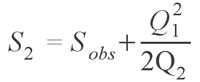
Although the Chao 1 estimator works for abundance data, often only occurrence data are available. There is another estimator, named conveniently Chao 2 (Chao 1987; Colwell and Coddington 1994), which uses occurrence data from multiple samples in aggregate to estimate the species diversity of the whole. This estimator is defined as:

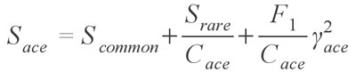
which is virtually identical to the Chao 1 estimator, with singletons (Q1) being species occurring in only one sample and doubletons (Q2) occurring in two samples. This estimator can also make use of the Chao 1 variance formula provided above, with the substitution of F1 and F2 for Q1 and Q2, respectively.

Chao and colleagues (Chao and Lee 1992; Chao et al. 1993; Lee and Chao 1994) have also published another pair of estimators, called the Abundance Coverage Estimator and the Incidence Coverage Estimator, which use abundance and occurrence based data sets, respectively. These estimators are much more complex; the Abundance-based Coverage Estimator takes the form

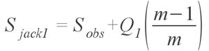
where Scommon are the species that occur more than 10 times in the sampling, Srare are those species which occur 10 times or less, Cace is the sample abundance coverage estimator, and finally ?ace is the estimated coefficient of variation for F1 for rare species (See Chazdon et al. 1998, for a full explanation and definition of the estimator). In simpler terms, the formula uses the number of rare species (>= 10) and the number of singletons (F1) to estimate how many more undiscovered species there might be. Although this formula is for the abundance estimator, virtually the same holds true for the incidence based estimator, except that instead of the species abundance, it uses the number of samples each species occurs in. Both of the coverage estimators have been found to give good results and are highly recommended (Chazdon et al. 1998; Hortal et al. 2006)

Another estimator provided is the Jackknife estimator, developed by Burnham and Overton (1978, 1979) originally for use with capture/recapture studies. The formula

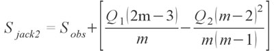
represents the first order version of the estimator; the variable m represents the total number of samples. Smith and van Belle (1984) also provided a second order variation, with the formula

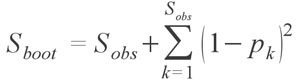
The second order Jackknife has shown to be one of the most effective estimators and may be the best estimator at the moment for highly sparse palaeontological collections since it is the least susceptible to sampling bias (Chazdon et al. 1998; Hortal et al. 2006).

Finally, for completeness I also provide the bootstrap estimator

developed by Smith and van Belle (1984). The bootstrap richness estimator has been generally regarded as one of the poorer species estimators, and Chazdon et al. (1998) in fact recommend against using it.

Though the various estimators vary greatly in their formulae, the functions within fossil take care of most of the nuances and generally require only one argument, that being a species occurrence matrix or species abundance vector or matrix.

>data(fdata.mat)
>chao1(fdata.mat)

[1]12.25

>jack1(fdata.mat) [1]12.98980

It is often best to use a number of these estimators in concert, as concurrence between their individual values can lend support to their results. Colwell (2009) has released a program for Windows called EstimateS which does exactly this; it can calculate multiple species estimators for a data set, along with their variances and a species accumulation curve. Since Colwell's program is so useful, it was used as a template to create the function spp.est(). The function has several important options, namely the number of randomizations and whether or not to use abundance data. The spp.est() function calculates a rarefaction curve, the Chao, Coverage Estimators and Jacknife, as well as standard deviations for all the estimates. As a default the function will run 10 randomizations of the data, however for more accurate estimates a much larger number of randomizations should be run. It should be noted that with a large data set and a large number of randomizations that the function may take a long time to complete. At this time, work has been undertaken to parallelize this function, enabling a large increase in processing time when using a multicore or multiprocessor system.