RESULTS
There are many ways to use data from controlled
surveys to explore patterns across space or through time in the fossil
assemblages themselves, or to test hypotheses concerning relationships of
paleontological trends to geological or geochemical evidence for
paleoenvironmental characteristics of the ancient landscapes and faunas. The
examples below are primarily exploratory in nature and are used to demonstrate
the potential benefits of standardized sampling. The results of these initial
analyses raise many questions that can be pursued in subsequent studies.
In the following sections, we use tallies and
proportions of the basic data collected for the biostratigraphic surveys, which
consist of identified specimens and tallies of turtle fragments and
unidentifiable scraps. Because specimens that were found in several or many
recently broken fragments were counted as one, the total number of specimens
should be a good approximation of the actual number of separate fossils for each
survey block or interval. We refer to this as NISP (number of identifiable
specimens; Badgley 1986a). The sample that was identifiable to taxon is NISPV
(identifiable at least to major vertebrate class) or NISPF (for
family or order), and the sample identifiable to skeletal region is NISPSK,
or NISPSKM for mammals only. In both cases, NISP probably is fairly
close to MNI, minimum number of individuals, or MNE, minimum number of elements,
respectively, given the wide dispersal of most of the specimens across the
surveyed outcrops (Badgley 1986a). However, we retain NISP as our basic unit of
analysis since we cannot test for MNI and MNE using data recorded on the survey
cards. A total of 121 survey blocks combined into 24 separate numbered surveys
(levels) were used in this analysis.
Fossil Productivity
 The number of fossil bones that were identified at
least to major vertebrate class (mammal, reptile, fish, bird) and/or to skeletal
element provides the basic data used for analysis of overall fossil
productivity. This combines the numbered specimens on the survey cards and the
“turtle tally,” which was used as a quick way to keep track of small fragments
of fossil turtle shell. The number of identified specimens (NISPV)
divided by the total number of search hours for each survey level (i.e., the
total for all surveyors who searched that level) gives a standardized measure of
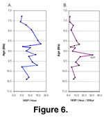
its fossil productivity (Pf; Table 1,
Figure 6A), with the mean value
for all survey levels of about 10 identifiable fossils per hour. Alternatively,
we could have used the area of outcrop covered in each survey to standardize
search effort; this was recorded on air photographs, but digitized information
for outcrop area is not yet available.
The number of fossil bones that were identified at
least to major vertebrate class (mammal, reptile, fish, bird) and/or to skeletal
element provides the basic data used for analysis of overall fossil
productivity. This combines the numbered specimens on the survey cards and the
“turtle tally,” which was used as a quick way to keep track of small fragments
of fossil turtle shell. The number of identified specimens (NISPV)
divided by the total number of search hours for each survey level (i.e., the
total for all surveyors who searched that level) gives a standardized measure of
its fossil productivity (Pf; Table 1,
Figure 6A), with the mean value
for all survey levels of about 10 identifiable fossils per hour. Alternatively,
we could have used the area of outcrop covered in each survey to standardize
search effort; this was recorded on air photographs, but digitized information
for outcrop area is not yet available.
We can make the assumption that the NISPV
/Hour (Pf) accurately represents the underlying fossil productivity
of each interval, but other variables may also affect the pattern of temporal
variation in productivity shown in Figure 6A. One of these is the thickness
(duration) of the stratigraphic interval being surveyed, which was variable
depending on search conditions. We tended to range vertically through thicker
intervals for surveys that were relatively unproductive but followed productive
strata laterally as far as possible, typically remaining within a relatively
thin stratigraphic interval. Dividing Pf by interval duration gives
a measure of productivity per 100 kyr (Table 1,
Figure 6B), which highlights the
narrow zone of exceptionally high productivity at KL01 and also the marked
drop-off in productivity upward in the sequence, after 7.6 Ma.
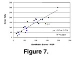 Unidentifiable scrap was tallied for each survey
interval, partly as a measure of the preservational state of surface fossils,
and partly to encourage surveyors to pick up and examine every fossil they
encountered. Not surprisingly, there is a high correlation between the number
of identifiable bones (NISPV) and scrap (Figure 7,
Table 1B). The
ratio is remarkably consistent throughout the survey samples, and we assume that
this reflects a combination of taphonomic processes operating prior to
deposition as well as fragmentation on the modern outcrop surfaces. In future
analyses it should be possible to test the role of modern outcrop topography on
the proportion of unidentifiable scrap using notes on the terrain and
photographs for each of the surveys. On average, for the portion of the Siwalik
sequence sampled using the surveys, one can expect to find a minimally
identifiable fossil for every 1.6 unidentifiable scraps, and a mammal specimen
identifiable at least to family for every 5 unidentifiable scraps. This metric
is a good indicator of the abundance of information for higher taxonomic levels
that is available in the eroded surface fossil assemblages of this fluvial
sequence. The proportion of museum-quality, collectible specimens found on
these surveys is much lower, compared to the high-density patches that
constitute formal localities.
Unidentifiable scrap was tallied for each survey
interval, partly as a measure of the preservational state of surface fossils,
and partly to encourage surveyors to pick up and examine every fossil they
encountered. Not surprisingly, there is a high correlation between the number
of identifiable bones (NISPV) and scrap (Figure 7,
Table 1B). The
ratio is remarkably consistent throughout the survey samples, and we assume that
this reflects a combination of taphonomic processes operating prior to
deposition as well as fragmentation on the modern outcrop surfaces. In future
analyses it should be possible to test the role of modern outcrop topography on
the proportion of unidentifiable scrap using notes on the terrain and
photographs for each of the surveys. On average, for the portion of the Siwalik
sequence sampled using the surveys, one can expect to find a minimally
identifiable fossil for every 1.6 unidentifiable scraps, and a mammal specimen
identifiable at least to family for every 5 unidentifiable scraps. This metric
is a good indicator of the abundance of information for higher taxonomic levels
that is available in the eroded surface fossil assemblages of this fluvial
sequence. The proportion of museum-quality, collectible specimens found on
these surveys is much lower, compared to the high-density patches that
constitute formal localities.
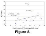 Fossil productivity (Pf) based on
biostratigraphic survey data can be compared with productivity based on number
of localities for approximately the same intervals (Figure 8,
Table 2). The
regression coefficient is positive but insignificant (R2 = 0.11), and
when the two obvious outliers are removed, it is also insignificant (R2
= 0.35). The productivity of a biostratigraphic survey thus is not a good
predictor of whether the interval will have rich concentrations of fossils,
indicating a partial disconnect between the presence of such patches and the
scatter of vertebrate remains between them. Interestingly, this suggests some
degree of continuity through time in the background of isolated fossil
vertebrate occurrences in the Siwalik deposits, contrasting with strong fluvial
and/or taphonomic controls on the presence or absence of notable bone
concentrations.
Fossil productivity (Pf) based on
biostratigraphic survey data can be compared with productivity based on number
of localities for approximately the same intervals (Figure 8,
Table 2). The
regression coefficient is positive but insignificant (R2 = 0.11), and
when the two obvious outliers are removed, it is also insignificant (R2
= 0.35). The productivity of a biostratigraphic survey thus is not a good
predictor of whether the interval will have rich concentrations of fossils,
indicating a partial disconnect between the presence of such patches and the
scatter of vertebrate remains between them. Interestingly, this suggests some
degree of continuity through time in the background of isolated fossil
vertebrate occurrences in the Siwalik deposits, contrasting with strong fluvial
and/or taphonomic controls on the presence or absence of notable bone
concentrations.
Skeletal Parts
The proportions of different skeletal parts in a
fossil assemblage can be used to infer the impact of taphonomic processes such
as transport and density-dependent destruction on the remains prior to burial
(Voorhies 1969;
Behrensmeyer 1991). The biostratigraphic surveys provide
standardized data for examining patterns through time in the representation of
different skeletal elements. Here we focus on teeth and axial elements
(vertebrae plus ribs), which represent the most and least dense elements in a
complete skeleton, respectively (Voorhies 1969;
Behrensmeyer 1975,
1988). Teeth
are generally regarded as the most “preservable” elements in the vertebrate
body, based on their density and mineralogy, which are particularly resistant to
chemical and biological break-down.
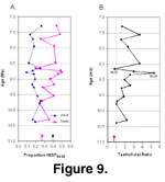 Teeth average 37% and axial parts 19% of
the total sample of 1282 mammalian records identifiable to body part (Figure 9,
Table 3), whereas they are 27% and 39%, respectively (excluding caudal
vertebrae), in the skeleton of a living ungulate (combination of bovid and equid). Relative to this standard, the Siwalik fossil assemblage is shifted
toward the denser, more preservable (and identifiable) elements. However,
variations through time show that some survey intervals preserved a much higher
proportion of teeth than others, suggesting differences in the taphonomic
filter(s) that controlled the preservation of vertebrae and ribs versus teeth.
Teeth average 37% and axial parts 19% of
the total sample of 1282 mammalian records identifiable to body part (Figure 9,
Table 3), whereas they are 27% and 39%, respectively (excluding caudal
vertebrae), in the skeleton of a living ungulate (combination of bovid and equid). Relative to this standard, the Siwalik fossil assemblage is shifted
toward the denser, more preservable (and identifiable) elements. However,
variations through time show that some survey intervals preserved a much higher
proportion of teeth than others, suggesting differences in the taphonomic
filter(s) that controlled the preservation of vertebrae and ribs versus teeth.
Based on studies in modern ecosystems and
laboratories, non-random variations through time in axial versus tooth
frequencies shown in Figure 9 could result from changes in: 1) levels of
pre-burial biotic processing of skeletons, i.e., carnivore and scavenger
pressure (Behrensmeyer 1993,
2002); 2) degrees of fluvial reworking of the
original bone assemblages, with increased reworking resulting in proportionately
fewer axial elements (Voorhies 1969;
Behrensmeyer 1991); 3) contributions of
channel versus floodplain deposits to the surface fossil assemblages recorded in
the biostratigraphic surveys; more durable body parts, especially teeth, would
be expected if channel deposits are the primary source of the fossils for any
given level. In the biostratigraphic survey data, teeth are consistently
dominant through the sequence, except for three intervals where they drop close
to a 1:1 ratio relative to axial elements. There is an unusual dominance of
teeth at about 8.8 Ma (survey ML06), followed by a drop to an unusually low
proportion at 8.7 Ma (ML05). Both of these extremes are in the Malhuwala Kas
area, ~15 km southwest of Kaulial and Ratha Kas where most of the surveys were
done. It is possible that variations in search conditions or original position
on the alluvial plain contribute to the differences in the ML samples. If we
ignore these two points, the ratio in Figure 9B shows a slight trend toward
increased tooth dominance upward in time, which corresponds to the sedimentological shift toward more mountain-proximal (buff), higher energy
fluvial systems in the Dhok Pathan Fm. of the Kaulial Kas section (Behrensmeyer
and Tauxe 1982). This suggests that the overall tooth versus axial pattern
reflects degree of fluvial reworking rather than other possible causes listed
above, but further work is needed to test this hypothesis.
Major Vertebrate Groups
Most paleontological collecting efforts focus on
one vertebrate class or size category (e.g., macro-mammals) and pay less
attention to associated fossils from other groups such as fish and reptiles. Therefore, the proportions of major vertebrate groups in most catalogued
inventories are biased by collecting practices and cannot be used to examine the
proportions of these groups in the source assemblages. Such information can be
important, however, for instance as a general indicator of aquatic versus
terrestrial habitats in fossil-preserving environments and overall taphonomic
(and potentially ecological) dominance of the different types of vertebrates. Standardized sampling also provides a means of examining and comparing these
variables at different times and places in the vertebrate record.
 In the Siwalik biostratigraphic survey data,
mammal remains average 71% and reptiles 28% of the recorded sample, whereas fish
are very rare (0.4%; Figure 10,
Table 1, and
Table 4). The near absence of fish is
unexpected, since many of the depositional environments were clearly aquatic and
occasional beds of abundant fish remains occur throughout the sequence. It is
probable that this pattern represents a taphonomic bias against the preservation
of fish remains in the Siwalik fluvial system. Apparently there were few robust
forms, such as armored catfish, whose remains would likely survive as fossils
and also be recognized on the biostratigraphic surveys. Of the documented
reptilian remains, 88% are chelonian, 8% crocodyloid, and the remainder snake,
lizard, and unidentifiable reptile. Most of the chelonian remains are ornamented
shell fragments from the family Trionychidae, which are the common
“soft-shelled” aquatic turtles, but tortoise and other smooth-shelled fragments
also occur.
In the Siwalik biostratigraphic survey data,
mammal remains average 71% and reptiles 28% of the recorded sample, whereas fish
are very rare (0.4%; Figure 10,
Table 1, and
Table 4). The near absence of fish is
unexpected, since many of the depositional environments were clearly aquatic and
occasional beds of abundant fish remains occur throughout the sequence. It is
probable that this pattern represents a taphonomic bias against the preservation
of fish remains in the Siwalik fluvial system. Apparently there were few robust
forms, such as armored catfish, whose remains would likely survive as fossils
and also be recognized on the biostratigraphic surveys. Of the documented
reptilian remains, 88% are chelonian, 8% crocodyloid, and the remainder snake,
lizard, and unidentifiable reptile. Most of the chelonian remains are ornamented
shell fragments from the family Trionychidae, which are the common
“soft-shelled” aquatic turtles, but tortoise and other smooth-shelled fragments
also occur.
The relative abundance of reptiles versus mammals
through time (Figure 10) shows an initial decline from RH02 through KL04, which
coincides with the transition from the channel-dominated blue-gray fluvial
system of the Nagri Fm. to the more floodplain-dominated buff fluvial system of
the Dhok Pathan Fm. (Behrensmeyer
and Tauxe 1982; Barry et al. 2002). The
anomalous peak in reptile versus mammal in KL03 is followed by a fairly constant
reptile abundance of around 20%. In both RK02 and KL03, the high relative
abundance of reptiles is accompanied by fish remains, suggesting that these two
levels sample more aquatic environments than the other levels, and also that the
decline in the reptiles in the early part of the sequence reflects a shift to
less aquatic conditions in the source deposits of the surface fossil assumblages.
Only one bird was recorded in the entire
biostratigraphic survey sample (on ML06). Since it is unlikely that we would
have missed many identifiable avian remains in the nearly 5000 bones examined
during the surveys, this indicates a strong taphonomic bias against the
preservation of such remains in the Siwalik fluvial system.
Equidae versus Bovidae
 An initial motivation for doing biostratigraphic
surveys was to increase the temporal resolution on important biostratigraphic
events, such as the appearance of “Hipparion” and the shift from equid to
bovid dominance through the Siwalik sequence. Biostratigraphic surveys in the
northern Potwar Plateau record the regional “Hipparion” appearance datum
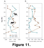
as shown in Figure 11. About two-thirds of the remains consist of teeth or
tooth fragments (Table 5), which should be similar in terms of the impact of
fluvial processes on their taphonomic histories. These remains also should be
equally identifiable to family. Equid molars are generally larger than bovid
molars, however, thus their abundance may be somewhat inflated in the preserved
remains and recorded samples. Overall, however, we regard the survey data for
equids and bovids as more or less isotaphonomic. Any biases in relative
abundance should be equivalent from level to level, and changes through time are
likely to reflect underlying ecological shifts in the diversity and/or abundance
of these two groups.
An initial motivation for doing biostratigraphic
surveys was to increase the temporal resolution on important biostratigraphic
events, such as the appearance of “Hipparion” and the shift from equid to
bovid dominance through the Siwalik sequence. Biostratigraphic surveys in the
northern Potwar Plateau record the regional “Hipparion” appearance datum
as shown in Figure 11. About two-thirds of the remains consist of teeth or
tooth fragments (Table 5), which should be similar in terms of the impact of
fluvial processes on their taphonomic histories. These remains also should be
equally identifiable to family. Equid molars are generally larger than bovid
molars, however, thus their abundance may be somewhat inflated in the preserved
remains and recorded samples. Overall, however, we regard the survey data for
equids and bovids as more or less isotaphonomic. Any biases in relative
abundance should be equivalent from level to level, and changes through time are
likely to reflect underlying ecological shifts in the diversity and/or abundance
of these two groups.
The biostratigraphic survey data begin close to
the “Hipparion” datum. There is an estimated 85 kyr between RK01, which
has no equid (i.e., species of the genus “Hipparion”) specimens, and
RK02+DH01+DH02 with five equid specimens. Biostratigraphic surveys in other
regions plus the locality data provide further support for a first appearance
datum (FAD) at 10.3 Ma (Barry et al. 2002). Based on their frequency in the
sample identifiable to mammalian family, the abundance of equid remains rises
while bovid abundance falls sharply between 10.3 and 9.8 Ma.
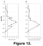 Equids
continue to dominate the mammalian macro-fauna until shortly before 8.5 Ma (Figure 11A,
Figure 12A), when bovids become more abundant. The ratio of equids to bovids shows
that equids reached their peak relative to bovids between 9.5 and 9.0 Ma (Figure 12A).
The same overall pattern is preserved in the teeth-only analysis (Figure 11B,
Figure 12B), except that the two lines are farther apart and equids are more
common than bovids until 7.7 Ma. We suggest that this results primarily from
higher survival and visibility of equid teeth on outcrop surface. Using all
documented skeletal remains (primarily appendicular) helps to boost tallies of
bovids relative to equids, perhaps because of more equivalent survival and
visibility levels for these post-cranial parts. Our working hypothesis,
therefore, is that the differences between Figure 11A-Figure 12A and
Figure 11B-Figure 12B are a
measure of durability and collecting bias between these two families rather than
a pre-burial taphonomic or ecological signal.
Equids
continue to dominate the mammalian macro-fauna until shortly before 8.5 Ma (Figure 11A,
Figure 12A), when bovids become more abundant. The ratio of equids to bovids shows
that equids reached their peak relative to bovids between 9.5 and 9.0 Ma (Figure 12A).
The same overall pattern is preserved in the teeth-only analysis (Figure 11B,
Figure 12B), except that the two lines are farther apart and equids are more
common than bovids until 7.7 Ma. We suggest that this results primarily from
higher survival and visibility of equid teeth on outcrop surface. Using all
documented skeletal remains (primarily appendicular) helps to boost tallies of
bovids relative to equids, perhaps because of more equivalent survival and
visibility levels for these post-cranial parts. Our working hypothesis,
therefore, is that the differences between Figure 11A-Figure 12A and
Figure 11B-Figure 12B are a
measure of durability and collecting bias between these two families rather than
a pre-burial taphonomic or ecological signal.
The overall pattern through time in Equidae versus
Bovidae, plus some of the shorter-term fluctuations in the sampled abundances
not related to teeth versus all identifiable parts, may indicate shifts in the
ecology of the alluvial plain favoring greater original abundance of one or the
other. There is no obvious environmental event at the “Hipparion”
appearance datum, and Barry et al. (2002) suggest that the faunal turnover at
around that time reflects biotic processes (e.g., competition). Our data
support this hypothesis, because partial competitive exclusion could explain the
reciprocal relationship of bovids versus equids shortly after 10.3 Ma, as well
as the low levels of bovid abundance for several million years thereafter. The
switch in abundance around 8.5 Ma also is not closely correlated with
environmental change, although there is evidence that patches of C4
vegetation may have been present at this time (Morgan 1994;
Barry et al. 2002). Turnover events at 7.8 Ma and 7.3-7.0 Ma, which are based on the overall Siwalik
faunal record and linked to environmental changes, are not obviously correlated
with the equid versus bovid trends in Figure 11-Figure 12.
Mammalian Families
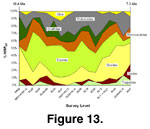 Eight major groups of macro-mammals dominate the
Siwalik paleocommunity. Their relative abundances in the biostratigraphic
survey sample are represented in Figure 13 (Table 6
and Table 7). Although most of
these taxa have been identified based on teeth, they are not necessarily as
isotaphonomic as bovids and equids. For example, a single proboscidean or
rhinoceros tooth can produce a large number of identifiable fragments,
especially compared with smaller artiodactyl teeth. Thus, the proportions of
the different groups in the survey samples are not a fair representation of
their original relative abundances. As in the case of the plots of equid versus
bovid abundance, however, these biases should be relatively constant from
interval to interval. The rare mammalian taxa found on the surveys include
aardvark, primate, chalicothere, carnivore (including hyena) and rodent, which
are grouped as “other” in Figure 13.
Eight major groups of macro-mammals dominate the
Siwalik paleocommunity. Their relative abundances in the biostratigraphic
survey sample are represented in Figure 13 (Table 6
and Table 7). Although most of
these taxa have been identified based on teeth, they are not necessarily as
isotaphonomic as bovids and equids. For example, a single proboscidean or
rhinoceros tooth can produce a large number of identifiable fragments,
especially compared with smaller artiodactyl teeth. Thus, the proportions of
the different groups in the survey samples are not a fair representation of
their original relative abundances. As in the case of the plots of equid versus
bovid abundance, however, these biases should be relatively constant from
interval to interval. The rare mammalian taxa found on the surveys include
aardvark, primate, chalicothere, carnivore (including hyena) and rodent, which
are grouped as “other” in Figure 13.
Overall there is moderate consistency in the
proportions of the eight major groups, and nearly all continue in the
paleocommunity through a time span of 3 Ma. Giraffes disappear from the sample
between 8.0 and 7.7 Ma, and equids become dominant, mostly at the expense of
bovids, shortly after their appearance (see also
Figure 11). There is an
interesting peak in giraffe abundance at 9.3 Ma (KL03), which coincides with the
period of maximum equid dominance, as well as unusual numbers of turtles
(Figure 11,
Table 1). There also are a large number of fossil localities at
this level (Table 2), including the Sivapithecus face site. This
suggests that KL03 had somewhat different fluvial conditions and perhaps less
seasonally dry habitats than other intervals. Another intriguing pattern is the
increase of tragulids and suids in the youngest intervals (after 7.9 Ma),
coinciding with the decline of giraffes and equids. Stable isotopes indicate an
important transition toward more intensely monsoonal climate and C4
vegetation starting around 7.3 Ma (Quade et al. 1989), and tragulid extinctions
were part of the major faunal turnover between 7.3 and 7.0 Ma (Barry et al.
2002). It is interesting that shortly before that time, tragulids were still
prominent members of the Siwalik paleocommunity.
