| |
USING THE STAGE
AMOR3 recognizes the presence or absence of a microfossil in a field of the slide only when the specimen resides in or close to the center of a particular field. For this reason, slides must be prepared accordingly, and specimens must be located near the center of a field in the slide. The second prerequisite for a successful operation of the program for keel-view analysis is that specimens are pre-oriented in approximate keel position. This conditioning was chosen in order to keep the complex problem of specimen orientation as simple as possible.
Single-Specimen Mode and Automeasurement Mode
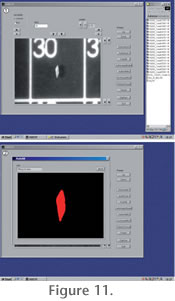 The AMOR software has two modes: A single-specimen mode, where individual specimens can be addressed manually (i.e., by driving the x and y gliding and tilting axes by mouse-clicks), and an auto-measurement mode for automated batch orientation and imaging of specimens in a slide. In the single-specimen mode, functions like specimen centering, up and down movements of the focus, autofocussing, zooming, translational and tilt movements, image rotation, and image capturing can be launched in any desired sequence (see
Figure 11.1-11.2). The AMOR software has two modes: A single-specimen mode, where individual specimens can be addressed manually (i.e., by driving the x and y gliding and tilting axes by mouse-clicks), and an auto-measurement mode for automated batch orientation and imaging of specimens in a slide. In the single-specimen mode, functions like specimen centering, up and down movements of the focus, autofocussing, zooming, translational and tilt movements, image rotation, and image capturing can be launched in any desired sequence (see
Figure 11.1-11.2).
In the auto-measurement mode these steps are automated. In this mode, a special panel allows flagging specimens individually for automated treatment of a selected range of fields in the slide. Alternatively, the entire slide can be processed at once. Also in this mode individual functions can be selected by check-boxes. Examples are the inclusion or exclusion Autorotation (keel view only, see above), or the manner how the software shall respond to runtime-errors (i.e., continue or interrupt for manual interaction). Upon launching the auto-measurement mode, the system moves to the first field that was previously selected, autocenters the specimen, focuses automatically, starts the pitch and roll tilting movement until the ideal position is attained, zooms up to the maximum possible magnification, focuses again, rotates the specimen vertically (only possible in keel view), captures the image, and saves it to a disc into a pre-defined directory. Grey-level images are written in Tiff format and have a size of 640 x 480 pixels, with 256 grey-levels per pixel. Thereafter, the system advances to the next field and repeats the sequence until all fields are treated.
In addition to the images produced by the scan, a text file is generated to
record the image names to reduce the scanning time per slide movement from one
row to the next occurs in a meander-like manner. Next to the images a text file is generated, which records the image names together with the corresponding magnifications for each image taken. This "list of files" can later be used in combination with external MorphCol programs (Knappertsbusch 2004) to automatically extract outline coordinates and to convert them from pixels to micrometers. During operation, a logging file records the successful treatment of each field, the magnifications, and the tilting positions. If an error occurs, it is logged as well, and the system abandons the actual field to advance to the next field.
For a slide containing 60 specimens in keel-position and with the motor-zoom function enabled, AMOR needed 86 minutes to process in auto-measurement mode. If the motor-zoom is disabled (in this case the magnification remains constant throughout scanning of the entire slide) the system is even faster. This rate of image collection is fast and outcompetes any experienced manually operating person.
Image Collection and Post-Processing
 Upon termination of AMOR3, the user has a collection of grey-level images with foraminiferal shells in perfect keel or spiral/umbilical view together with the necessary information about the magnification taken for every image. Upon termination of AMOR3, the user has a collection of grey-level images with foraminiferal shells in perfect keel or spiral/umbilical view together with the necessary information about the magnification taken for every image.
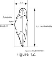
The collected grey-level images need to be further processed to outline coordinates in micrometers, from which geometric parameters like size or shape descriptors can be derived. In our case outline analysis of the shells in keel view has been proven to contain the most useful shape information (see
Figure 12).
 There exist a great number of software packages in the public domain (see, for example, the morphmet discussion list) for this task. In our case a suite of self-written Fortran programs is used, which are described in
Knappertsbusch (1998) and
Knappertsbusch (2004), in combination with public domain software NIH-Image or ImageJ from Wayne Rasband. A special macro "automation" written in NIH-Image (see
Brown 2007) for a listing) helps to quickly batch-process grey-level images to binary black and white images prior to outline extraction (note: binary images could, theoretically, already be exported to disc during the real-time image processing while orienting the specimens. This bears potential for abbreviating the entire process of image collection and post-processing in the future. There exist a great number of software packages in the public domain (see, for example, the morphmet discussion list) for this task. In our case a suite of self-written Fortran programs is used, which are described in
Knappertsbusch (1998) and
Knappertsbusch (2004), in combination with public domain software NIH-Image or ImageJ from Wayne Rasband. A special macro "automation" written in NIH-Image (see
Brown 2007) for a listing) helps to quickly batch-process grey-level images to binary black and white images prior to outline extraction (note: binary images could, theoretically, already be exported to disc during the real-time image processing while orienting the specimens. This bears potential for abbreviating the entire process of image collection and post-processing in the future.
 At this stage of development, this possibility has not implemented yet in order to keep development steps (i.e., image collection vs. post-processing) as easy as possible.
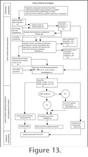
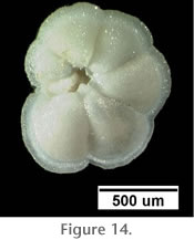
Figure 13 illustrates a work-flow scheme for the post-processing for Globorotalia menardii (Figure 14) applied in
Knappertsbusch (2007). At this stage of development, this possibility has not implemented yet in order to keep development steps (i.e., image collection vs. post-processing) as easy as possible.
Figure 13 illustrates a work-flow scheme for the post-processing for Globorotalia menardii (Figure 14) applied in
Knappertsbusch (2007).
Precision and Repeatability of the System
The quality of morphometric data after imaging with AMOR depends on many factors: Illumination, image quality, thresholding and segmentation in binary images, precision of the x and y translational and tilting motors, correct camera calibration (i.e., pixel to micrometer conversion as a function of magnification), calibration of the microscope magnification (i.e., precision of the mechanical drive of the zoom and the translation of the zoom-movement into a numerical magnification factor). All these factors were carefully checked prior to routine applications, under controlled conditions of a darkened room (changing roomlight may alter the light conditions) and always using the same single specimen.
In AMOR thresholding can be adjusted during initialization by setting the illumination, diaphragm, and the polarizers. For better control, the diaphragm and the polarizers were labelled using a millimetre-paper stripe, so that identical settings can be reproduced. Too low illumination caused the binary image of the specimen to be eroded. However, it was observed that above a certain threshold this influence vanished. The camera calibration was performed using a 1 mm scale with 10 micrometer subdivisions. Calibration must be carried out for every objective used, at every magnification in horizontal and vertical directions in order to compensate for the various influences of chip-size of the camera and the properties of the frame grabber. Whenever the imaging system is modified (i.e., new objectives, different type of zoom-body or microscope, digital camera, C-mount, frame grabber, or another computer system) calibration must be renewed. The influence of polarizing filters (if inserted in the light path of the microscope) did not cause any changes in magnification factors, but caused a slight lateral shift of the image on the computer monitor that does not affect morphometric measurements.
 The magnification of the zoom-body of the Leica MZ6 as a function of the rotation angle of the zoom knob follows an exponential relationship. This relationship was found empirically by attaching a millimetre-paper stripe around the zoom knob and so measuring the angular positions at the indicated magnifications (i.e., 0.63x, 0.8x, 1.0x, 1.6x, 2.0x, 2.5x, 3.2x, and 4.0x). The detailed results of these experiments are described in supplements No. 6 and 7 of MorphCol (Knappertsbusch 2004). Applying this relationship allowed the calculation of magnifications at any zoom-position when using the stepping motor. The magnification of the zoom-body of the Leica MZ6 as a function of the rotation angle of the zoom knob follows an exponential relationship. This relationship was found empirically by attaching a millimetre-paper stripe around the zoom knob and so measuring the angular positions at the indicated magnifications (i.e., 0.63x, 0.8x, 1.0x, 1.6x, 2.0x, 2.5x, 3.2x, and 4.0x). The detailed results of these experiments are described in supplements No. 6 and 7 of MorphCol (Knappertsbusch 2004). Applying this relationship allowed the calculation of magnifications at any zoom-position when using the stepping motor.
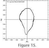
Figure 15 and
Figure 16 illustrate the precision of AMOR after repeated orientation, imaging, processing, and extraction of outlines to cartesian coordinates of the same single specimen for several times: In
Figure 15 the test specimen was 15 times oriented, imaged, and processed to outlines in auto-measurement mode and using the motorized zoom.
 In
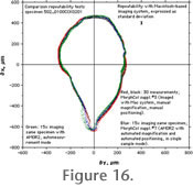
Figure 16 three different repeatability tests are compared to each other: In Test 1 the same specimen was oriented 30 times by hand using the hemi-spherical stage shown in
Figure 1 and using Nih-image software on a Macintosh-based digital imaging system. In
Figure 16 three different repeatability tests are compared to each other: In Test 1 the same specimen was oriented 30 times by hand using the hemi-spherical stage shown in
Figure 1 and using Nih-image software on a Macintosh-based digital imaging system.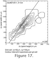 In Test 2, the same specimen was automatically oriented 15 times using AMOR2 and with the automated zoom enabled, but in single-specimen mode. In Test 3 of
Figure 17, the test specimen was oriented using AMOR2 and with the automated zoom enabled, but in auto-measurement mode. In general, there is reasonable agreement of the test series among and between each other. In Test 2, the same specimen was automatically oriented 15 times using AMOR2 and with the automated zoom enabled, but in single-specimen mode. In Test 3 of
Figure 17, the test specimen was oriented using AMOR2 and with the automated zoom enabled, but in auto-measurement mode. In general, there is reasonable agreement of the test series among and between each other.
Statistical analysis of the areas in keel view from 38 orientation measurements done for the same specimen have shown that the standard error with respect to the mean area in keel view is 0.233% and 3.438% with respect to the difference between the minimum and maximum area of the 38 investigated shells (which is 0.0263mm2, see
MorphCol supplement No. 8,
Knappertsbusch 2004).
|