METHODS
Data Acquisition
For this analysis, biogeographic ranges of taxa were reconstructed at both the species and genus level at the temporal resolution of stratigraphic sequence of
Holland and Patzkowsky (1996) using Geographic Information Systems (GIS). The geographic ranges of rhynchonelliform brachiopods were reconstructed because analyses of these organisms are expected to produce the most accurate range reconstructions for Cincinnatian taxa.
Brachiopod fossils are among the most diverse and abundant fossils that are present in all Cincinnatian depositional environments, and most can be identified to species based on external skeletal morphology (Meyer and Davis 2009). High sampling density and accurate species identifications reduces undersampling and other errors potentially associated with range reconstruction (see
Rode and Lieberman 2004). Brachiopods lived on or borrowed shallowly within the seafloor, thus their fossils distribution likely reflects their actual living distribution accurately on the outcrop scale (Kidwell and Flessa 1996), the scale at which these analyses are conducted. As noted above, storm processes, which affected Cincinnatian benthos, did not result in significant lateral transport of skeletal material (Frey 1987;
Barbour 2001). Moreover,
Finnegan and Droser (2008) noted that storm deposits have a higher proportion of local taxa than unreworked beds because they concentrate rare taxa in the resulting lag. Consequently, although these storms impacted the sediment, storm reworking produced biodiversity data that are more complete than non-reworked deposits.
Data required to reconstruct geographic ranges consist of geographically and temporally restricted species occurrence data. These data include species identification, precise latitude and longitude coordinates of the collection locality, and stratigraphic information to place the species occurrence within the correct stratigraphic sequence. Species occurrence data were collected from museum collections, targeted field work, and the
Paleobiology Database. Collections at the Cincinnati Museum Center, Miami University Limper Museum, and the Ohio State University Orton Geological Museum were examined. At each museum, specimens were inspected by the author in order to verify (or correct) species identifications. Species identifications followed published identification keys (Davis 1998,
Feldmann 1996) and published synonymies (e.g.,
Walker 1982). Taxa known to be problematic or for which current consensus opinion questions their taxonomic validity (e.g., Platystrophia unicostata and Rafinesquina fracta ) were excluded from the database. Specimens with stratigraphic or geographic information that could not be resolved to sequence or precise location (e.g., Late Ordovician, Cincinnati Region) were necessarily excluded from the dataset. Museum data
were supplemented by a download of data, primarily the dataset of
Holland and Patzkowsky (2007), from the Paleobiology Database and field work targeted to fill in gaps in data coverage. The final species occurrence database includes 1490 unique species occurrence data points for 49 brachiopod species in 21 genera across all six depositional sequences (Figure 1,
Table 1,
Table 2,
Appendix 1).
Range Reconstruction
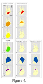 Geographic ranges were calculated in two ways using GIS. The first method estimates the area of a geographic range by creating a minimum spanning convex hull to enclose all known occurrence points for a taxon (see examples in
Figure 4). Using this method, all known taxon occurrence sites are enclosed by a polygon with the fewest possible number of sides, then the area of that polygon is calculated in ArcGIS (ESRI 2008). This method has been successfully employed with Devonian brachiopods and bivalves (Rode and Lieberman 2004), Devonian phyllocarids (Rode and Lieberman 2005), and Cambrian arthropods (Hendricks et al. 2008). Step-by-step instructions for this method are presented in
Stigall Rode (2005) and
Stigall (2006). Although the polygon method provides the most parsimonious estimate of a taxon's geographic range, it is potentially sensitive to underestimation of a taxon's range due to undersampling or overestimation of geographic ranges that were not laterally continuous (see
Stigall Rode and Lieberman 2005). Therefore, geographic ranges were also estimated using a distance method based on the maximum linear extent between two points of known taxon occurrence, a method previously employed by
Hendricks et al. (2008). To further reduce the sensitivity of the results to sampling bias, analyses were calculated at both the species and genus levels. The 49 species analyzed comprised 21 genera. Of these, twelve invasive genera and one Maysvillian restricted genus were monotypic within the study. There are currently no published phylogenetic analyses for relationships of Cincinnatian brachiopods. The monophyly of some genera, such as Strophomena and Platystrophia, have been questioned (Zuykov and Harper 2007; Leighton, personal comun., 2009), while some species, such as Dalmenella meeki, are known to be assigned to genera to which they do not belong (Jin, personal comun., 2009). As species are a primary unit of evolutionary innovation, whereas genera represent systematists's opinions of related but potentially non-monophyletic groups of species, the discussion below will focus primarily on species-level patterns. Generic level data will be used to assess and support the relative strength of the pattern at multiple taxonomic levels.
Geographic ranges were calculated in two ways using GIS. The first method estimates the area of a geographic range by creating a minimum spanning convex hull to enclose all known occurrence points for a taxon (see examples in
Figure 4). Using this method, all known taxon occurrence sites are enclosed by a polygon with the fewest possible number of sides, then the area of that polygon is calculated in ArcGIS (ESRI 2008). This method has been successfully employed with Devonian brachiopods and bivalves (Rode and Lieberman 2004), Devonian phyllocarids (Rode and Lieberman 2005), and Cambrian arthropods (Hendricks et al. 2008). Step-by-step instructions for this method are presented in
Stigall Rode (2005) and
Stigall (2006). Although the polygon method provides the most parsimonious estimate of a taxon's geographic range, it is potentially sensitive to underestimation of a taxon's range due to undersampling or overestimation of geographic ranges that were not laterally continuous (see
Stigall Rode and Lieberman 2005). Therefore, geographic ranges were also estimated using a distance method based on the maximum linear extent between two points of known taxon occurrence, a method previously employed by
Hendricks et al. (2008). To further reduce the sensitivity of the results to sampling bias, analyses were calculated at both the species and genus levels. The 49 species analyzed comprised 21 genera. Of these, twelve invasive genera and one Maysvillian restricted genus were monotypic within the study. There are currently no published phylogenetic analyses for relationships of Cincinnatian brachiopods. The monophyly of some genera, such as Strophomena and Platystrophia, have been questioned (Zuykov and Harper 2007; Leighton, personal comun., 2009), while some species, such as Dalmenella meeki, are known to be assigned to genera to which they do not belong (Jin, personal comun., 2009). As species are a primary unit of evolutionary innovation, whereas genera represent systematists's opinions of related but potentially non-monophyletic groups of species, the discussion below will focus primarily on species-level patterns. Generic level data will be used to assess and support the relative strength of the pattern at multiple taxonomic levels.
The areal extent of the outcrop belt shifts significantly in both size and location among sequences. As discussed above, Cincinnatian strata were deposited along a depositional ramp, which prograded northward through time. Furthermore, strata are now exposed along a structural arch. Therefore, the oldest sequences outcrop more centrally along the arch whereas the younger sequences occur both toward the northern and more distal regions of the arch (Figure 1). In order to meaningfully compare temporal patterns among sequences, these variations in outcrop availability must be accommodated. Therefore, calculated geographic ranges were normalized by outcrop extent for each time slice. Areal ranges were normalized by dividing the observed range by the area of the minimum convex hull digitized for all species occurrence data in the database for a single sequence (Table 1,
Table 2). Maximum linear extents were similarly normalized by dividing by the maximum linear extent between any pair of species occurrences within a single sequence (Table 3,
Table 4).
A second standardizing procedure, dividing the raw geographic range estimate by the number of species occurrence points used in the range estimation, was also undertaken (Appendix 2). Results of statistical analyses conducted with data normalized by occurrence points were congruent with those of the area standardized data. (Appendices 3-4, 6-9). Normalizing by outcrop extent is less heavily influenced by sampling bias or sampling intensity. Therefore, results of analyses conducted using the area standardized range values will be discussed in the text.
Statistical Analyses
To assess whether certain types of species responded differently to the invasive regime, species were categorized into four groups: (1) species native to the Cincinnati region which did not persist beyond the Maysvillian Stage, (2) species native to the Cincinnati region which were extant in the Maysvillian and carryover into the Richmondian, (3) species that evolved in the Richmondian from Cincinnati natives, and (4) extrabasinal invaders (Table 1,
Table 2,
Table 3,
Table 4). For generic analyses, only categories 1, 2, and 4 were used. Because phylogenetic relationships are almost entirely unknown for Cincinnatian brachiopods, species group membership was coded in two ways. In the first coding strategy (indicated in
Table 1,
Table 2,
Table 3,
Table 4), category 3 includes all Richmondian species assigned to a genus that existed Cincinnati during the Maysvillian, and category 4 includes all Richmondian species assigned to a genus absent from Maysvillian strata of the Cincinnati region. This coding scheme assumes that all of the Richmondian members of a Maysvillian genus occur in Richmondian strata due to speciation within the basin and that none of these species migrated to Cincinnati as part of the Richmondian
Invasion. While this interpretation is the most parsimonious, it may not be
accurate for all species in the category; some species of native genera may be. This may have arrived
in the Cincinnati region as part of the invasion, particularly true for species
of Strophomena. This genus is absent from C3 strata of the Cincinnati region (Table 1), which may represent extirpation from the basin. Furthermore, some Richmondian species, notably Strophomena planumbona, occur in the Maquoketa Formation on the west side of the basin during the C3 sequence (Leighton, personal commun., 2009). Therefore, a second coding strategy was employed in which all Richmondian species of Strophomena were treated as invasive rather than as native descendants. For generic analyses, Strophomena was treated as a carryover taxon in the first coding strategy. In the second coding strategy, C1 and C2 Strophomena were treated as Maysvillian restricted genus while the C4-C6 Strophomena were treated as an invasive genus.
Two sets of statistical analyses were conducted based on the estimated geographic ranges. The first assessed differences in geographic range versus taxon group; whereas the second set analyzed changes in geographic range by sequence. Differences in geographic response by taxon group were analyzed using one-tailed t-tests, and temporal patterns were assessed using analysis of variance (ANOVA). All analyses were conducted with Minitab 15 (Minitab Inc. 2007). Analyses were conducted separately for the two taxon group coding strategies.