Global dental ecometrics

Computational biomes: The ecometrics of large mammal teeth

Esther Galbrun, Hui Tang, Mikael Fortelius, and Indrė Žliobaitė

Article number: 21.1.3A
https://doi.org/10.26879/786
Copyright Palaeontological Association, January 2018

Author biographies
Plain-language and multi-lingual abstracts
PDF version

Submission: 26 May 2017. Acceptance: 17 January 2018

{flike id=2122}

ABSTRACT

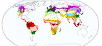
As organisms are adapted to their environments, assemblages of taxa can be used to describe environments in the present and in the past. Here, we use a data mining method, namely redescription mining, to discover and analyze patterns of association between large herbivorous mammals and their environments via their functional traits. We focus on functional properties of animal teeth, characterized using a recently developed dental trait scoring scheme. The teeth of herbivorous mammals serve as an interface to obtain energy from food, and are therefore expected to match the types of plant food available in their environment. Hence, dental traits are expected to carry a signal of environmental conditions. We analyze a global compilation of occurrences of large herbivorous mammals and of bioclimatic conditions. We identify common patterns of association between dental traits distributions and bioclimatic conditions and discuss their implications. Each pattern can be considered as a computational biome. Our analysis distinguishes three global zones, which we refer to as the boreal-temperate moist zone, the tropical moist zone and the tropical-subtropical dry zone. The boreal-temperate moist zone is mainly characterized by seasonal cold temperatures, a lack of hypsodonty and a high share of species with obtuse lophs. The tropical moist zone is mainly characterized by high temperatures, high isothermality, abundant precipitation and a high share of species with acute rather than obtuse lophs. Finally, the tropical dry zone is mainly characterized by a high seasonality of temperatures and precipitation, as well as high hypsodonty and horizodonty. We find that the dental traits signature of African rain forests is quite different from the signature of climatically similar sites in North America and Asia, where hypsodont species and species with obtuse lophs are mostly absent. In terms of climate and dental signatures, the African seasonal tropics share many similarities with Central-South Asian sites. Interestingly, the Tibetan plateau is covered both by redescriptions from the tropical-subtropical dry group and by redescriptions from the boreal-temperate moist group, suggesting a combination of features from both zones in its dental traits and climate.

Esther Galbrun. Department of Computer Science, Aalto University, P.O. Box 15400, FI-00076 Aalto, Finland. esther.galbrun@aalto.fi
Hui Tang. Department of Geosciences, University of Oslo, P.O. Box 1022, University of Oslo, 0315-Oslo, Norway. hui.tang@geo.uio.no
Mikael Fortelius. Department of Geosciences and Geography, University of Helsinki, P.O. Box 64, FI-00014 University of Helsinki, Finland. mikael.fortelius@helsinki.fi
Indrė Žliobaitė. Department of Computer Science, University of Helsinki, P.O. Box 68, FI-00014 University of Helsinki, Finland; Department of Geosciences and Geography, University of Helsinki, P.O. Box 64, FI-00014 University of Helsinki, Finland. indre.zliobaite@helsinki.fi

Keywords: ecometrics; redescription mining; dental traits; large mammals; data mining

Final citation: Galbrun, Esther, Tang, Hui, Fortelius, Mikael, and Žliobaitė, Indrė. 2018. Computational biomes: The ecometrics of large mammal teeth. Palaeontologia Electronica 21.1.3A 1-31. https://doi.org/10.26879/786
palaeo-electronica.org/content/2018/2122-global-dental-ecometrics

Copyright: January 2018 Palaeontology Association.
This is an open access article distributed under the terms of Attribution-NonCommercial-ShareAlike 4.0 International (CC BY-NC-SA 4.0), which permits users to copy and redistribute the material in any medium or format, provided it is not used for commercial purposes and the original author and source are credited, with indications if any changes are made.
creativecommons.org/licenses/by-nc-sa/4.0/

INTRODUCTION

Understanding the relationship between organisms and their environments over time and space is one of the key questions in paleobiology. Knowing how present-day communities relate to their environments allows for the computational capture of these patterns of associations, which can help to better understand fossil communities in the past and the processes that drive evolutionary change. Here we use data mining techniques to extract and analyze such associations from modern-day global data.

The approach relies on the assumption that the ways in which communities relate to their environment and survive in it persist over time, even though communities change as taxa evolve. The older the assemblage, the more different the taxonomic composition of the assemblage tends to be from present-day composition. Yet functional traits of taxa, governed by the laws of physics, chemistry and physiology, are likely to be similar in the present and in the past. For example, animals that run tend to leave the same pattern of skeletal architecture, i.e., long limbs (Reed, 2013).

Ecometrics is a computational methodology that focuses on identifying and modeling functional relationships between traits of organisms and their environments (Fortelius et al., 2002; Eronen et al., 2010c). Ecometrics can be used for reconstructing past climate and environments (Eronen et al., 2010b; Meloro and Kovarovic, 2013; Saarinen, 2015; Sukselainen et al., 2015; Fortelius et al., 2016), understanding evolution of faunal communities (Eronen et al., 2009), analysing macroevolution patterns (Schnitzler et al., 2017) and understanding the functional relationships between organisms and their environments (Eronen et al., 2010a; Lawing et al., 2012; Liu et al., 2012; Polly and Head, 2015; Zliobaite et al., 2016; Barr, 2017). Different traits have been explored for ecometric analyses. For plants, leaf shapes have been considered (Wolfe, 1995; Traiser et al., 2005). For animals, considered traits include teeth (Eronen et al., 2010a; Liu et al., 2012; Meloro and Kovarovic, 2013; Polly and Head, 2015; Fortelius et al., 2016; Zliobaite et al., 2016), limbs and locomotion (Polly and Head, 2015; Barr, 2017; Levering et al., 2017), skeletal traits (Lawing et al., 2012), as well as body mass (Meloro and Kovarovic, 2013). Traditionally, the term ecometrics refers to the analysis of animal traits. Conceptually similar approaches for modeling relationships between the distribution of species and the physical environment via functional traits are known in ecology as species distribution models (Elith and Leathwick, 2009), or four-corner models (Brown et al., 2014). However, such models have a different objective: given environmental conditions, the goal is to estimate the likelihood of the presence, or the abundance, of species. In paleobiology and paleoecology modeling the focus is reversed: species distribution data are available and the goal is to reason about the physical environment. Canonical correspondence analysis of community composition (Legendre and Legendre, 2012) constitutes yet another computational task, where the goal is to identify environmental gradients for species distributions directly from the occurrence data, without the proxy of functional traits.

The goal of our study is to identify global patterns of association between dental traits of large herbivorous mammals and their environments in an ecometric way, that is, by analyzing dental trait distributions across communities. The analysis uses a data mining approach called redescription mining (Ramakrishnan et al., 2004), which in our study aims at describing geographic localities in terms of two alternative vocabularies: dental traits of occurring taxa on one hand and environmental conditions on the other. With this approach, we obtain a set of redescriptions ranked by accuracy, among which we identify common trends. We then analyze those trends across climatic zones. This approach differs from common ecometric modeling, where global models are constructed with the aim of accurately predicting climate based on the traits of species communities (see e.g., Liu et al., 2012). Instead, redescription mining identifies associations between dental traits and climate which hold locally. The approach is conceptually similar to identifying biomes, that is, large ecological areas defined by abiotic factors such as climate, relief, geology and soils, hosting animals and plants adapted to their environment. For this reason, we refer to the redescriptions that we identify through a data-driven process as computational biomes.

DENTAL TRAITS AND DATA ARRANGEMENT

Animal teeth serve as an interface to obtain energy from food. Among other functions, teeth help to acquire energy more efficiently by mechanically breaking down the food before digestion. For animals to survive in their environments, their teeth need to be well suited for processing available and obtainable food. Plant matter is particularly demanding on teeth and chewing due to the necessity to break a high number of tough cell walls containing plant fibers, as well as to the abrasiveness of plant materials (which can also be due to extrinsic particles). As the types and characteristics of plant matter available vary between localities, from the poles to the equator, from forests to deserts, the shapes and dental characteristics of mammalian teeth, especially of herbivorous mammals, vary along these dimensions. Thus, since teeth are calibrated for eating particular types of plants, and the kinds of plants that grow in different locations depend on the prevailing environmental conditions, dental traits of herbivorous mammals are expected to be highly dependent on the environment and can therefore help to characterize it.

Dental Traits Scoring: Functional Crown Types

Remarkably, many functional characteristics of the teeth of herbivorous mammals, such as crown height, scale isometrically with the size of the animal (see Ungar, 2014, for a recent review). For example, a hyrax (body size 2–5 kg) and a black rhino (body size 800–1400 kg) have almost identically shaped teeth, only scaled to their body size. This scaling property makes it possible to directly describe animal communities in terms of the distribution of their dental characteristics.

Hypsodonty is the most common such characteristic. It describes how tall a tooth is in relation to its width or length. The more hypsodont, the more durable to wear the tooth. The mean hypsodonty of a community has been widely used as a proxy for precipitation (Fortelius et al., 2002; Eronen et al., 2010a; Kaiser et al., 2013; Fortelius et al., 2016). The proxy resolves precipitation primarily due to hypsodonty being common in grasslands and rare in (temperate) forests, and grasslands in turn being typically drier than forest habitats. There are several factors to this effect, and they are fortunately correlated in their effects: food quality, food toughness and degree of contamination with extrinsic particles. All of these tend to increase on the closed-open axis (Fortelius et al., 2002).

Another functional characteristic of the teeth of herbivorous mammals commonly used to estimate climatic conditions is the presence of lophs (Liu et al., 2012; Fortelius et al., 2016; Zliobaite et al., 2016). Globally, the higher the average loph count of the community, the lower the mean annual temperature is expected to be (Liu et al., 2012). High average loph counts denote the presence of topographically prominent longitudinal lophs, an uncommon feature among hippos, suids and among large shares of primates and elephants. In fact, rhinos as well as part of the primates possess teeth with only one longitudinal loph. Northern latitudes, which happen to be cooler, feature almost none of these groups, so that the average lophedness is higher in the north. As a result, high average loph counts carry a signal of lower mean annual temperatures.

In this study, we use the functional dental traits scoring scheme introduced in Zliobaite et al. (2016), which quantitatively describes morphological characteristics of molar teeth such as hypsodonty, lophodonty and their structural properties. A detailed list of traits is provided in the next paragraph. This set of dental traits was explicitly designed for capturing molar shape and the main functional traits of worn occlusal surfaces of the molar dentition. The scheme is built on a modular system called crown types introduced by Jernvall (1995). The system has been designed to be generally applicable to all living and fossil herbivorous mammals, regardless of phylogenetic origin, size or morphology of the chewing apparatus. The dental traits are intended to be independent of body size, given the diet. Further details about the design and rationale behind this scoring scheme can be found in the publication by Zliobaite et al. (2016).

There are seven variables describing dental traits, divided into four categories as indicated in Table 1. These traits apply to the dominant upper molar from the functional perspective. The default position is upper M2, and M2 should be referred to when all upper molars have the same functional traits. The purpose is to always capture the significant traits of the entire molar dentition. For suids, M3 is clearly the tooth that changes most during evolution and the one that responds to functional selection, therefore M3 should be used to determine the scores for suids. Scoring with M2 instead would miss most of the functional differences between taxa, except for the early suid species where M3 is regular, and it does not matter whether M2 or M3 is used.

Hypsodonty characterizes the height of a tooth, as mentioned earlier, while horizodonty characterizes the length of the functional surface. Hypsodont and hypsohorizodont, respectively, qualify high-crowned teeth and horizontally elongated teeth. Both traits are meant to capture the relative durability of a tooth with respect to dental wear. Acute lophs and obtuse lophs, respectively, designate sharp edges and blunt edges across the chewing direction. Pointed structures on a tooth are called cusps. Structural fortification of cusps refers to the structures being reinforced by local enamel thickening, by folding or both. When structural fortifications are present, the cusps typically remain prominent while the rest of the teeth wear down. Occlusal topography refers to the surface of a tooth being flat or non-flat (rugged). Coronal cementum is a substance covering a tooth to support its strength and durability.

Figure 1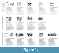 presents a set of examples with various combinations of the seven dental traits for selected living and fossil genera, noting that scoring of all traits is not always possible from pictures only. Scoring is at the level of species or higher taxa. Sometimes individual specimens of the same species may vary, especially in terms of occlusal topography or cementum. In such a case, the most common score across the inspected specimens is assigned for the species.

This functional dental traits scoring scheme is used to describe numerically the characteristics of teeth related to their durability, strength, wear resistance and wear patterns.

Data Sources

In an ecometrics study typically a site is the unit of analysis. Sites may correspond to physical places (e.g., national parks), ecologically defined regions (e.g., ecoregions) or geographic units (e.g., identified by placing a grid on a map). To extract ecometric patterns, we need to know environmental characteristics and trait distributions at each site.

Our study builds on three datasets: taxa occurrence data at localities (Sites × Taxa), dental traits of taxa (Taxa × Traits) and climate variables at localities (Sites × Climate). Traits data are assigned at the species level, considering that the traits are the same for all individuals within a species (Taxa × Traits). Therefore, this study does not require observation or measurement of the traits of particular animals occurring at localities, only to know which species occur at which localities (Sites × Taxa).

Species occurrence data come from the list of the International Union for Conservation of Nature (IUCN; https://www.iucn.org). Table 2 lists the different orders and families represented in the data, with the number of sites where they occur in each continent. Climate variables come from the WorldClim dataset (http://www.worldclim.org/), which builds on extrapolated observations from weather stations. The datasets of species occurrences and of climate variables (Sites × Taxa and Sites × Climate, respectively) have been compiled by M. Lawing and colleagues (Lawing et al., 2016), communicated by J. Eronen. We used square grids of 50 by 50 km size as units of analysis, the finer resolution for the mammals occurrence and the climate available from the data sources. The occurrence data are based on ranges defined by the IUCN. Inherently, since animals are moving, occurrence ranges of large mammals can rarely be more precisely defined than in the order of tens of kilometers. This resolution is sufficient for our purpose of identifying and analyzing global relations between dental traits of animal communities and climate.

The dental traits dataset has been compiled by the authors (M. Fortelius and colleagues) and is available online at http://www.helsinki.fi/science/now/ecometrics. Most hypsodonty scores come from Liu et al. (2012). The new traits data, together with all the reused datasets, the parameter settings for the mining algorithm and the algorithm outputs are available online at https://github.com/zliobaite/teeth-redescription.

From the three data sources that we are using, the occurrence data are expected to be the most uncertain, since these data are based on expert inferred and observed ranges of occurrences. The precision of such data for large mammals is inherently limited to a scale of at least a few kilometers. Indeed, since animals move, presence and abundance may vary overtime. Dental traits data are at the species level and are expected to be precise according to the scoring scheme used. Climate data are based on observations, but observations stations do not cover the world uniformly, therefore the data are interpolated (by the data provider). Bearing in mind the origin of the occurrence data and the climate data, we perform our analysis at a quite a coarse resolution (50×50 km units), expecting both the occurrence data and the climate data to be reliable enough for our purpose at this level of approximation. It would not be sensible to zoom in to a finer resolution.

Data Aggregation

Given the taxa occurrence data at localities (Sites × Taxa) and the dental traits of taxa (Taxa × Traits) we build the traits at sites dataset (Sites × Traits). Traits at sites can in principle be described by any descriptive characteristic of data distribution. Here we use the arithmetic mean.

The original Functional Crown Type scoring scheme (Zliobaite et al., 2016) has seven dental trait variables, five of which are binary and two (HYP and HOD) are ordinal. We converted both ordinal variables into binary variables for individual species. In other words, we replaced variable HYP, which takes value 1, 2 or 3, by three binary variables Hyp1, Hyp2 and Hyp3, such that, for a given species, the new variable Hyp3 equals 1 if variable HYP took value 3 for the species and equals 0 otherwise. Similarly for variables Hyp1 and Hyp2 with HYP values 1 and 2, respectively. We replaced variable HOD by three binary variables Hod1, Hod2 and Hod3 in the same way.

Then, for each site and each trait, we took the mean of the binary trait variable over the taxa that occur at the site. This corresponds to calculating what fraction of the taxa occurring at the site displays the considered trait. It results in trait distribution data at sites (Sites × Traits), where the dental trait variables describing sites are all numeric variables in the range [0,1]. For instance, the entry corresponding to location #1152 and dental trait Hod1 indicates what fraction of the taxa occurring at this location have brachyhorizodont teeth (i.e., for which variable HOD takes value 1 in the original Functional Crown Type scoring scheme).

Following this aggregation, we have a pair of datasets, (Sites × Traits) and (Sites × Climate), with matching sites characterized, respectively, by dental trait variables and climate variables. Two such datasets form the input of the redescription mining algorithm described in Section “Computational Data Analysis Method: Redescription Mining,” which returns a collection of redescriptions, highlighting associations between the dental traits variables, the climate variables and sets of locations.

Figure 2 sum 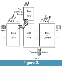marizes the processes of aggregating taxa occurrences and dental traits over locations, and of extracting redescriptions. The three initial datasets are represented by rectangles with a double border while the rectangle representing the aggregated dataset has a single border.

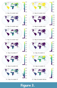
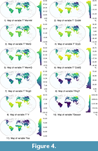
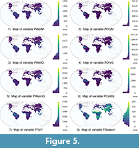
The input of the redescription mining process is the pair of datasets (Sites × Traits) and (Sites × Climate). These datasets contain 11 dental traits variables (Hyp1 to CM) and 19 bioclimatic variables (T^~Y to PColdQ), respectively (see Table 3). The variables are plotted on world maps in Figure 3, Figure 4, Figure 5 (high-definition zoomable versions of all the maps appearing in this paper are available online at https://github.com/zliobaite/teeth-redescription).

We discard locations with two taxa or fewer, considering that the data in such locations are too limited for the distribution of dental traits to be informative. This leaves us with 28887 locations, about 57% from the total 50365. Therefore, the input to the mining algorithm consists of a pair of real-valued matrices of sizes, respectively, 28887×11 and 28887×19.

COMPUTATIONAL DATA ANALYSIS METHOD:
REDESCRIPTION MINING

Introduced by Ramakrishnan et al. (2004), redescription mining is a data mining technique, which can be applied to data from various domains. For instance, using socio-political survey data, a recent study by Galbrun and Miettinen (2016) considered the candidates to the Finnish parliamentary elections, looking for typical associations between their political opinions and attributes from their personal profiles (including age, education level and party membership, among others).

The high-level objective of redescription mining is to find several distinct descriptions for the same set of entities and to identify sets of entities that share several distinct descriptions.

In the study mentioned above, the entities were individual persons, more specifically the electoral candidates. In the present study, entities are geographic localities, also referred to as sites. Each locality is a square on the world map.

Descriptions, also referred to as queries, express constraints on the values that variables might take. For instance, when considering electoral candidates, the query might require their age to fall within a particular range and specify that they must currently be an elected representative. In the present study, considering localities, queries might require the maximum monthly precipitation to fall within a given range and require the prevalence of particular traits or the occurrence of certain species. By requiring that a particular binary variable (e.g., elected status, species occurrence) be true or that a numerical variable (e.g., age, temperature, trait prevalence) take value in a specified range, such queries implicitly select a subset of entities, those entities which satisfy the constraints. For this reason, we say that the query is a description of those entities.

Redescription mining aims to identify pairs of queries such that the entities selected by either one are roughly the same. In our setting, one query will be expressed over bioclimatic variables, and the other query will be in terms of dental traits of occurring large herbivorous mammals. Each such pair will provide two different ways to characterize (roughly) the same sites. In other words, it provides alternative descriptions of those sites, hence the name redescription.

In general, redescription mining takes as input a collection of entities and two sets of variables. Neither the subsets of entities nor the queries are given a priori, both are discovered concurrently and automatically. The output of redescription mining is a set of query pairs, such that the two queries of each pair share a relatively large fraction of entities on which they hold. The queries of each pair describe a subset of entities. In that sense, redescriptions constitute local models, each one only applying to the entities in the associated subset. Therefore, redescription mining can be considered to be a local approach. This is in contrast to conventional predictive modeling methods, such as regression modeling, which can be considered to be global approaches, as they aim at building global models, optimizing for associations that hold as well as possible for all entities.

The subsets of sites thus characterized form regions, which can conceptually be compared to biomes—large ecological areas defined by abiotic factors such as climate, relief, geology and soils with animals and plants adapting to their environment. In this study, the results of redescription mining can thus be thought of as computational biomes. Note that redescription mining as employed here does not in any direct way enforce geographic continuity. However, the subsets of sites tend to form contiguous regions as a result of continuity in the conditions and of spatial autocorrelation between the variables.

What Redescriptions Are

Entities can be described using different vocabularies. Redescriptions identify alternative, nearly equivalent, ways for describing entities, in the form of pairs of descriptions over two different vocabularies, respectively.

Descriptions, also referred to as queries, are logical statements over the variables. The support of a query q is the set of entities that satisfy it, denoted as supp(q). In other words, the support of a query is a list of sites where the climatic variables or the dental traits match the conditions specified in the query. Then, a redescription is a pair of queries, one over each of the two sets of variables, satisfied by roughly the same entities, that is, having similar supports. The support of a redescription is the subset of entities described by both queries. In other words, it is the intersection of the supports of the two queries. Overloading the notation, we denote the support of a redescription R = (q_a,q_b) as supp(R), which is such that

 

The similarity of the supports of the two queries that make up a redescription, also called the accuracy of the redescription, could be assessed using any existing set similarity measure. In redescription mining, the Jaccard coefficient is generally used for this purpose, because it is simple, intuitive and symmetric, in the sense that the two sets are considered in the same way. The Jaccard coefficient compares the number of elements common to both sets to the number of elements in their union. Formally, for two sets S_a and S_b it is defined as

Informally, we are trying to maximize the number of sites described by both queries while minimizing the number of sites described by only one of them. That is, we aim at finding queries that describe the same sites from different perspectives, not just in the sense that some of the sites they describe are the same, but so that the entire sets of sites described by the two queries are (roughly) the same. The Jaccard coefficient is well suited for this purpose, as it takes into account the sites that are described by either queries or both, but not the sites that are not described by either queries. We do not require any specific value of the coefficient to be reached, what constitutes a satisfactory value for the Jaccard coefficient depends on the data, that is, on the type and quality of the input, as well as on the context of the analysis.

In addition to being accurate, the redescriptions should be statistically significant. In particular, for a given redescription R = (q_a, q_b), we compute a p-value that indicates how likely it is that two subsets of entities X_a and X_b sampled independently with probabilities respectively

and

where n denotes the total number of entities in the dataset, have an intersection as large or larger than the observed support of the redescription, supp(R). This p-value can be computed using the following formula:

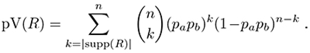The redescription is deemed non-significant if the p-value is larger that some threshold (typically 0.01 or 0.05).

As a practical example, consider the following query over bioclimatic variables:

We use Iverson bracket to specify satisfiability conditions, that is, in our case, the ranges in which the variables must take value. The query above selects sites where the value of T^~WarmQ is lower than 18.3, and the value of T^~ColdQ is lower than 6. In other words, it selects sites where the temperature averages below 18.3°C during the warmest quarter and below 6°C during the coldest quarter.

Now, take the following, slightly more complex query over dental traits:

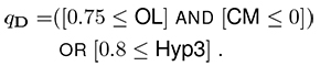
A site satisfies this query if among the taxa occurring there, either more than three-quarters have teeth with obtuse lophs and none has teeth with coronal cementum, or more than 80% are hypsodont.

In the dataset used in this study, which contains 28887 sites in total, we find that 8590 sites satisfy this distribution of dental traits among taxa, while 7374 sites satisfy the climatic profile specified by q_C, i.e., |supp(q_D)|=8590 and |supp(q_C)|=7374. Among these sites, 6286 satisfy both queries. Hence, we have

We consider this similarity to be satisfactory and the pair (q_D, q_C) to be an accurate redescription, which we refer to as Rx. The p-value computed with the marginal probabilities 8590/28887=0.297 and 7374/28887=0.255 equals

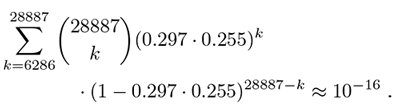
That is, the p-value is essentially zero, and the redescription can be considered significant at significance levels both 95% (threshold 0.05) as well as 99% (threshold 0.01). In summary, the support size, accuracy and p-value of the redescription are |supp(Rx)|=6286, J(Rx)=0.65 and pV(x)=0.00.

How Redescriptions Are Built

Given a collection of entities and two sets of variables characterizing them, the aim of redescription mining is to automatically find pairs of queries that constitute accurate redescriptions.

Since its introduction, several algorithms have been proposed for this task. Some are based on exhaustively searching groups of frequently co-occurring values (Gallo et al., 2008). Others learn predictive models, namely classification trees, from which queries are then extracted (Ramakrishnan et al., 2004; Zinchenko et al., 2015). Yet others rely on empirically engineered searches to build the queries step by step (Gallo et al., 2008; Galbrun and Miettinen, 2012). In this study, we used the REREMI algorithm (Galbrun and Miettinen, 2012) for obtaining redescriptions. This algorithm is able to handle numerical data, in contrast to previous algorithms, which were designed to work exclusively on Boolean data, i.e., data that contain only two distinct values, usually denoted by true and false. The REREMI algorithm provides a number of tuneable parameters allowing, for instance, to set thresholds on the size of the support of the output redescriptions and to control the length and complexity of their queries.

The analysis was carried out using SIREN (http://siren.gforge.inria.fr/main/), an interface that allows to automatically generate redescriptions with various algorithms, including REREMI, and to visualize and interactively edit the redescriptions (Galbrun and Miettinen, 2014). Initial parameters can be set based on domain knowledge, a priori expectations and requirements. The interface allows to automatically mine redescriptions and to then adjust the parameters in response to the results obtained, progressively refining them in successive rounds of interaction.

REREMI is a greedy algorithm (i.e., it makes a locally optimal choice at each iteration) that mines redescriptions by iteratively appending new variables to the current queries, at each step keeping the best candidates for further extension. In the initialization phase, the algorithm tests all variable pairs, in our case each dental trait variable with each bioclimatic variable, aiming to form simple redescriptions. In the extension phase, the algorithm then considers these simple redescriptions and extends them by appending additional variables to either of the queries. At each step, given the current candidate redescription, the algorithm considers each variable in turn and computes the extension that would result from appending it to the candidate. The best resulting extensions are selected, to be extended further in the next steps. The selection is driven primarily by the accuracy, that is, the algorithm chooses the extensions that yield the greatest increase in Jaccard coefficient, while remaining within the constraints specified by the parameters. When no improvement in the accuracy measure can be achieved, if the maximum query length is reached or if some support requirement is broken, this process stops and the best redescription is returned. Initial simple redescriptions are expanded in turns, from the most accurate, i.e., most promising ones to the least accurate, while cycling through the different variables in order to promote diversity in the results.

For example, four extension steps are shown in Table 4, leading from a redescription involving only the two variables OL and T^-ColdM to a more accurate redescription involving three dental trait variables and two bioclimatic variables.

An additional step, appending Hyp2 to the dental traits query, produces redescription R4, which will be discussed later. At each step, the algorithm not only tests all available variables for extension but also determines the threshold constraining the variables, setting the lower and upper bounds for T^~WarmQ, respectively, to 0.1 and 21.6 in the last step of the example above, for instance. To do so, a search is performed over possible values for the thresholds, exploiting the fact that only a limited number of values actually need to be tested rather than all values taken by the variable.

For a more detailed discussion of the REREMI mining algorithm, the interested reader is refered to Galbrun and Miettinen (2012).

Data Analysis Process

Input. The input of the redescription mining process is the pair of datasets (Sites × Traits) and (Sites × Climate), or in more concrete terms two real-valued matrices of sizes respectively 28887×11 and 28887×19, as explained in Section “Data Aggregation.” All variables are listed in Table 3.

Output. The output of the mining process is a collection of redescriptions, i.e., of pairs of queries, one over dental trait variables and one over climate variables, respectively, each associated to the sets of locations satisfying the queries. We look for such pairs that have a high accuracy, i.e., a high Jaccard coefficient between the respective supports of the queries constituting the pair.

Parameters. The mining process can be adjusted by tuning a range of parameters, described in more details in the SIREN user guide (http://siren.gforge.inria.fr/help/). The most important parameters are constraints on the support size and on the type of queries, which are set as follows.

For our analysis, we required that at least 1% of locations satisfy both queries (MinSuppIn), and that at least 60% of locations satisfy neither of the queries (MinSuppOut). In other words, the intersection of the supports of the two queries (the support of the redescription) and their union must contain at least 1% and at most 40% of all locations, respectively. Indeed, to be informative, the areas described should neither be too large, corresponding to overly generic redescriptions, nor too small, corresponding to overly specific redescriptions, and we found these thresholds to provide a good balance.

Also, we let dental trait queries involve up to four variables, while restricting the climate queries to at most two variables. We adjusted the maximum number of variables per queries based on our experience of modelling the associations between dental trait distributions and climatic variables in Kenyan national parks (Zliobaite et al., 2016). In our experience, a combination of three or four dental traits was sufficient to generate reasonably accurate estimates. Further increasing the number of variables can only marginally improve estimates, but can make interpretation of the results much more complicated. We limited the number of environmental variables to two, since the climate variables essentially measure two physical phenomena, temperature and precipitation.

Technically, both conjunctions and disjunctions can be used on either of the dental traits, the climate queries or both. Conjunctions are more strict since they require both conditions to be true, for example: high percentage of hypsodont and low percentage of flat teeth. Disjunctions are more inclusive, since only one of the conditions needs to be true, for example: high percentage of hypsodont or low percentage of flat teeth. As we strived for redescriptions that are reasonably easy to analyze and interpret, we did not allow disjunctions to appear simultaneously in both queries of a redescription. For the same reason, we also did not allow negations to appear in the queries.

Computational analysis process. We mined redescriptions using the dental traits and climate variables described earlier. The goal of the experiment was to find what associations between dental trait distributions and climate are best supported in this dataset.

We obtained 384 redescriptions in total, with accuracies ranging from 0.68 down to 0.03, and support sizes between 6694 and 289 locations. In other words, the obtained redescriptions cover between 23.17% and 1% of the total 28887 locations, with the smaller support sizes matching the minimum support threshold MinSuppIn. All obtained redescriptions and their variants that we report here had p-value essentially zero, well below the significance threshold. Hence, all the reported redescriptions can be considered to be statistically significant and we do not report the p-value for each one separately. The mining process took about 50 minutes to complete on a commodity laptop.

The obtained redescriptions can be ranked by their accuracy, and can be filtered based on whether they contain dental traits or climate variables of interest. Next, we will discuss a selection of the redescriptions mined automatically in the experiment. Specifically, we will present the ten redescriptions with the highest accuracy and three redescriptions involving high values for the precipitation seasonality, since they are a representative subset of high quality results covering the different areas. In addition, we present variants of some of these redescriptions, obtained through automatic and manual edits of the dental traits queries, which allow us to delve deeper in the analysis of the conditions specified by the queries.

Implications for the analysis of the fossil record. Models of current situations also inform how we study the past, providing frameworks and hypotheses to be tested using historical experiments (McGuire and Davis, 2014). Apart from explaining associations between dental characteristics of herbivorous mammals and their habitats existing at present, the identified redescriptions could potentially be applied to reconstruct the palaeoclimate and its major climate types based on fossil mammal assemblages, following the principles of ecometric analyses. Given a collection of redescriptions extracted, as we do here, from present traits and climate data, and given fossil assemblage data, the approach would work as follows. After computing the trait distributions for fossil assemblages, one could consider each redescription in turn, looking for localities where its dental queries hold. One can then expect that the climate in such localities might have corresponded to the conditions specified in the climatic query of the redescription.

Modern days may not always accurately reflect the past, but one reassuring feature of ecometric approaches is that they rely on functional traits averaged over faunal communities, instead of presence or absence of particular species or particular traits. While almost all dental traits as such can be found in almost all environments, what matters is which traits are common for which environments. Therefore, one can hope that rare cases will be averaged over and most common general patterns driving evolution across communities (Jernvall and Fortelius, 2002; Hannisdal et al., 2017) will surface.

While mechanically simple, such a projection of the redescriptions in the past requires further investigations, for instance, to propose systematic ways in which to evaluate the ability of the patterns to generalize to unseen data, to reconcile the diverging projections that may arise from different redescriptions, and to estimate the reliability of the resulting climate predictions. In particular, the probability that a projected redescription holds could be computed based on its accuracy and support in the modern data. Hence, the second step, the projection of the redescriptions in the past, is not entirely straightforward. Neither is the first step, the extraction of the redescription from modern data, on which we focus in this study.

ANALYSIS OF RESULTING REDESCRIPTIONS

The most accurate redescriptions selected according to the analysis protocol specified earlier are denoted as R1–R10 and listed in Table 5. These 10 redescriptions show the highest Jaccard coefficients among all those returned by the algorithm.

We can see that the dominant dental characteristics in the resulting queries are hypsodonty and obtuse lophs, closely followed by acute lophs and structural fortification. Horizodonty, cement and occlusal topography appear more rarely.

The climate queries of the top 10 redescriptions either contain only temperature variables or combine temperature and precipitation variables, typically highlighting limits, ranges or seasonality. The climate queries in the top four redescriptions (R1–R4) and in the last redescription (R10) include only temperature variables, specifying ranges of temperatures, or referring to the limits of warmth and cold. The remaining five queries (in R5–R9) each combine one temperature variable and one precipitation variable. In the latter cases, the temperature variable typically concerns the range (TIso) or the seasonality (TSeason). The precipitation variables capture either annual precipitation (PTotY) or precipitation of the wettest quarter (PWetQ).

Hypsodonty and lophedness are the most dominant dental traits. These variables have been shown to be good proxies for the global temperature and precipitation (Liu et al., 2012). It has also been demonstrated that, at least in Africa, dental traits of herbivorous animals better reflect limiting climatic conditions than average conditions (Zliobaite et al., 2016), which manifests in variables that specify limits being overrepresented in the climate queries.

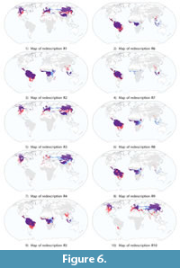Interestingly, lower limits on precipitation, which would capture arid climates, do not appear in the top 10 redescriptions. Aridity is usually expressed as a function of rainfall and temperature (Food and Agriculture Organization of the United Nation, 1989). Aridity indeed constitutes an important climatic constraint, limiting the availability and quality of vegetation, and in turn imposing functional demands on the teeth for feeding on such vegetation (Strömberg, 2002). The absence of lower limits on precipitation can be explained by the geographic coverage of the top 10 redescriptions, as visualized in Figure 6. We can see that all redescriptions cover primarily either a boreal-temperate moist zone in the northern hemisphere (R1, R3, R4, R10) or a tropical moist zone near the equator (R2, R5–R9). We observe that the top redescriptions do not involve lower limits on precipitation. This makes sense because the lack of precipitation is not a factor limiting the productivity of the environment in either of the two zones. Indeed, in the north, the primary productivity of the environment is mainly limited by temperature, not precipitation, as inferred from Lieth (1975) and the temperature also controls nitrogen availability in this region (Melillo et al., 1993). On the other hand, in the tropical forest regions, net primary productivity (NPP) is generally limited by moisture, nutrients (Cleveland et al., 2011) and disturbances (e.g., fire). Competition for light can also lead to self thinning of forests and thus also limit NPP. Thus, since they do not cover the arid regions in the tropical latitudes, it makes sense that the top redescriptions do not involve lower limits on precipitation.

Next, we analyze the top ten redescriptions, separately for the boreal-temperate moist zone and the tropical moist zone. Then, to cover all major climatic zones of the globe, we specifically look for redescriptions characterizing a tropical-subtropical dry climate among the results and discuss them in Section “Tropical-Subtropical Dry Zone”.

Boreal-Temperate Moist Zone

The redescription with the highest accuracy, R1, indicates that sites with less than 33% of mesodont species, no horizontal elongation of teeth, less than 6% species having acute lophs and more than 75% of species having obtuse lophs can be described by temperatures of the warmest quarter lower than 18.3°C and temperatures of the coldest quarter lower than 6°C. These temperature limits capture the temperate-cold climate, including cold mountain climate (e.g., the Tibetan Plateau and the Rocky Mountains). This redescription holds in North America, Europe and Eastern Siberia. It represents temperate climate in Europe, boreal climate in northern Eurasia and North America. Indeed, these habitats are dominated by boreal forest species with typically selenodont teeth (crescent-shaped cusps), most of those teeth are low-crowned and have lophs, that are characteristic dental traits for browsers (Popowics and Fortelius, 1997). Redescription R1 gives a plausible description of the northern boreal-temperate forest habitats (preferable needleleaf tree cover). Exceptions to these conditions include Europe, due to strong human activity, and the Tibetan Plateau, which is at a notably higher elevation (around 4500 m on average) than the rest of R1 and thus mainly contains tundra and herbaceous cover. We explore these conditions further, by deriving variants of this redescription.

Table 6 presents 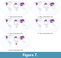four variants of redescription R1, denoted as R1a–R1d. The corresponding maps are visualized in Figure 7. By manually removing Hyp2 from the dental traits query of R1 we obtain redescription R1a. Then, we completely delete the dental trait query and let the algorithm automatically find new queries over dental traits to match the climatic query, but restricting the search space. More specifically, we deactivate some variables so that the algorithm does not use them when building extensions. After deactivating horizodonty variables (Hod1, Hod2 and Hod3) as well as the acute lophs variable (AL) we obtain variants R1b. Further deactivating the hypsodonty variable (Hyp2) which occurred in the original query, we obtain variants R1c and R1d.

By comparing R1 and R1a, we notice that removing the requirement on the share of mesodont species (Hyp2) has only a small impact on the accuracy. We can see from the visualization of dental traits in Figure 3 that hypsohorizodont species appear primarily in Africa. Thus, the requirement for all species to be brachyhorizodont keeps the dental query in R1 away from Africa, but a similar effect is already achieved by the requirement of a low share of acute lophs. Comparing R1 and R1b shows that removing the horizodonty and acute lophs constraints (Hod1 and AL, respectively) has a larger impact. Indeed, the term requiring no horizodontal elongation of teeth plays an important role in redescription R1. Horizontal elongation is only present in elephants and African suids, which generally do not occur in the northern hemisphere where the climatic conditions of this redescription (low temperatures with a large difference between seasons) are satisfied. This holds for the modern day, but it may not hold, for instance, looking back into the Pleistocene where proboscidians with horizontally elongated molars lived in very cold climates. In the modern data the mean hypsodonty and lophedness conditions do apply in some parts of Africa, thus, the horizodonty condition mostly contributes to excluding the African locations from the support. Evidence of this is visible from the map of R1b in Figure 7 where the African localities, which do not satisfy the cold climate query, join the support of the dental traits query (drawn in red) as a consequence of removing the horizodonty variable.

Further variants R1c and R1d introduce restrictions on the percentage of high hypsodonty (Hyp3) and on the presence of cementum (CM). Conceptually, these restrictions are similar to requiring no horizontal elongation,because they eliminate warm climate localities. Again the effect is mostly to exclude Africa, where savanna habitats with a high percentage of grass demand high hypsodonty (Strömberg, 2002), and high hypsodonty is strongly correlated with the presence of cementum (Zliobaite et al., 2016).

Overall, redescriptions of the boreal-temperate moist zone most commonly emphasize a high number of species having obtuse lophs and a lack of hypsodonty, which is in line with expectations from the ecology and ecometrics perspectives (Liu et al., 2012). The boreal-temperate moist zone is dominated by several species of deer, which have lophed teeth but never become hypsodont (Heywood, 2010). The lophedness of molar surface reflects the tooth’s cutting capacity per unit action (Kay and Hiiemae, 1974). A high cutting capacity in combination with low hypsodonty suggests high functional demands without increased tooth wear, which is characteristic of cool and vegetated habitats, where the major available plant food during the cold season consists of tough, but not very abrasive structural plant parts.

Tropical Moist Zone

The second redescription from the top 10 list, R2, describes sites near the equator in Africa, South America and Asia, as can be seen from the map in Figure 6.

The climate query describes a hot climate subject to several variations. The maximum temperature of the warmest month (T⁺WarmM) is required to be between 17.7 and 35.8°C, while the isothermality (TIso)—which is the ratio of the mean diurnal temperature range to the annual temperature range, i.e., TIso=T^~RngD/TRngY—is required to be greater than 67%. It implies a low seasonality in the temperatures, that is, the annual temperature range being almost as limited as the daily temperature range.

The dental query of R2 is more complex than for the boreal-temperate forest area, since it consists of two parts connected by a disjunction (i.e., an “OR”). The query requires either a large share of brachydont species and a small share of species with obtuse lophs, or a small share of species with flat occlusal topography and a small share of hypsodont species. This disjunction in the query is needed to describe the tropical moist zone globally, since the distribution of dental traits in the African part is quite different from their distribution in South America and Asia.

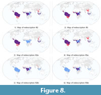
Table 7 lists redescription variants of R2, namely R2a and R2b, obtained by manually splitting the dental traits query into two components. The two components correspond to the dental trait distribution of South America and Asia (R2a) on one hand, and Africa (R2b), on the other hand, as can be seen from the corresponding maps in Figure 8.

The dental query of R2a combines a requirement for a large share of brachydont species and a small share of species having obtuse lophs. This redescription characterizes the tropical moist zones in South America and Asia, where the share of hypsodont species is very low. South America used to have hypsodont species (Madden, 2014), but now all are extinct.

The dental query of R2b requires that taxa with flat occlusal topography constitute a low but non-zero fraction of present taxa, and that hypsodont taxa constitute no more than about a third of present taxa. A large share of hypsodont species suggests an environment dominated by grasslands (Strömberg et al., 2013). Characterizing the African habitats around the equator with flat topography and high hypsodonty, which primarily signal grass eating, suggests that the African rain forest environments include a small share of grassland adapted fauna, and perhaps include open canopy with grasses.

The sites covered by redescription R5 are similar to those covered by R2: rain forest areas around the equator in Africa, South America and Asia. While the climatic query of R2 required high temperatures and high isothermality (annual range of temperatures similar to diurnal range of temperatures), the climatic query of R5 also requires high isothermality but associated to high annual precipitation (between 613 and 6989 mm in total). We can see from the maps in Figure 6 that the areas satisfying R2 and R5 (drawn in purple) are very similar, with R5 being slightly more patchy in Africa. The main difference from the climatic perspective is that R2 covers the Somalian peninsula, while R5 does not, but this area is not supported by the dental queries of R2 nor of R5, so this region does not belong to the support of either redescription.

Similarly to R2, R5 can be split into two components. The resulting redescriptions, R5a and R5b, are listed in Table 7 and visualized in Figure 8. A central region of Africa is described by R5b, while another region of Africa, along with regions in South America and Asia are described by R5a. Interestingly, the support of R5 in Africa is divided into two parts, which was not the case with R2. This difference arises from the differences in variables involved in the dental traits query of R5 as compared to that of R2. Unlike in the variants of R2, the query of R5a imposes constraints on the presence of acute and obtuse lophed species, but puts no requirement on the presence of hypsodont species. Such a constraint would not be satisfied in South America and Asia, because of the absence of hypsodont species in those tropical forest areas. The query of R5b, the African redescription of the tropical forests, imposes constraints on the presence of obtuse lophs and on the presence of hypsohorizodont species. Hypsohorizodonty, that is, horizodontal elongation of teeth, is a characteristic currently present almost exclusively in Africa. It would be different in the past, for instance proboscidians lived in very cold climates in the Northern hemisphere in the Pleistocene and Holocene (Stuart et al., 2004).

Overall, the tropical moist zone is associated with the presence of acute and obtuse lophs, but not in very large shares. Lophed teeth are characteristic of forest species. Hypsodonty is not strongly necessary, as these habitats are very humid, even though hot, and provide plant food which is tough (Dominy et al., 2003), but not too abrasive and does not put high pressure on teeth durability. Indeed, the combination of low cutting capacity and low hypsodonty indicates a general lack of stress, such as herbivores may encounter in warm and humid conditions with a wide variety of edible plant parts available throughout the year (Liu et al., 2012). The tropical moist zone is the richest in species and can host forms that would not survive on fibrous food, because there is never a bad season in those environments.

Tropical-Subtropical Dry Zone

In order to obtain redescriptions complementing the geographic coverage of the top ten, we take a closer look at those that characterize regions with high precipitation seasonality. From the list of all 379 obtained redescriptions we select for further analysis the redescriptions with the highest accuracy and including high values for variable PSeason. These redescriptions cover the tropical-subtropical dry zone, as can be seen from Figure 9, which complements the two previously identified zones.

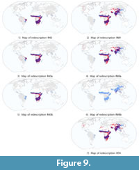In Table 8, we report redescriptions involving high values for variable PSeason, that is, redescriptions which describe areas with high precipitation seasonality. More specifically, we report the three most accurate such redescriptions returned by the main mining process. These redescriptions are ranked respectively 43th, 69th and 74th among the original results and hence denoted as R43, R69 and R74, respectively. The geographic areas, corresponding to those redescriptions, are visualized in Figure 9.

In addition to the precipitation seasonality, the climate queries in these redescriptions involve isothermality, temperature annual range and temperature seasonality, respectively. All these climate characterizations emphasize seasonality. Geographically, these queries mainly cover tropical Africa, excluding the rain forest areas near the equator, in addition to either patches in South America (R43), or patches in Central-South Asia, including India and the Tibetan Plateau (R69 and R74).

Interestingly, the Tibetan Plateau is included in R1 from the boreal-temperate moist zone, and also appears in the current group of redescriptions in R69 and R74. The climate query of R1 emphasizes seasonality and low level of temperature, which applies to the Tibetan Plateau, while R69 and R74 constrain the width of the temperature range without requiring any particular temperature, and also restrict the seasonality of precipitation, two conditions which apply to the Tibetan Plateau. The Tibetan Plateau is hence present in both zones. The climate over the Tibetan Plateau is cold and has high seasonality in temperature and precipitation. Because it includes the Tibetan Plateau, we cannot regard the current set of redescriptions as representing only the tropical-subtropical dry zone, but regard it as representing the climate with high seasonality in both tropical and temperate zones more generally. The remaining redescription, R74, involves the tropical-subtropical zone only.

The dental traits query of R43 requires the presence of a low fraction of brachydont and of hypsohorizodont species. Sites where either 96% of taxa are brachyhorizodont or 16.7% have obtuse lophs are also included in the support, through a disjunction. The conditions for horizodonty and obtuse lophs in the dental query of R43 require very precise values, and it is more likely an artifact in the data than a generic pattern. Therefore, we obtain simplified queries by dropping the inequalities associated with the two variables. Redescription R43a is obtained by removing the condition for the low share of brachyhorizodont taxa (0.96 ≤ Hod1 ≤ 0.96). Further removing the condition for obtuse lophs (0.167 ≤ OL ≤ 0.167) yields redescription R43b. The first removal has almost no impact on the accuracy and support of the redescription. The removal of the inequality associated with obtuse lophs, however, removes a patch in South America. The patch due to a precise value of lophedness seems to be a rather artificial construct, and we therefore believe that R43b constitutes a more informative representation than the original R43.

The dental traits query of R69 requires that among taxa present at the sites at least a third be hypsodont and less than 1% have acute lophs. Besides, sites where about two fifth of taxa or more are mesodont or about two fifth of taxa have structural fortifications of cups are included in the support through a disjunction.

Acute lophs combined with a relatively high hypsodonty, as well as structural fortification of cups have been associated with woody covered areas in arid tropical environments (Zliobaite et al., 2016). Interestingly, R69 also includes South Asia, as can be seen from Figure 9. We further investigate this redescription by splitting the dental traits query. Specifically, R69a and R69b result from keeping only the conjunction of hypsodonty and acute lophs and only the condition on structural fortifications of cups, respectively. We can see from Figure 9 that the structural fortification constraint applies mainly to the costal parts of India, and does not seem to hold generically across the areas supported by this redescription. R69a is a simplified version of R69, obtained by dropping the structural fortification and mesodonty constraints, which seems to hold generically across the African and Asian areas in question. This query suggests that the arid African areas are comparable in terms of their climate and dental characteristics to the South Asian areas. Climatically, the tropical arid region and South Asia are both affected by monsoonal climate. Therefore, both regions are characterized by high seasonality (Wang et al., 2014). The dental trait queries require relatively high hypsodonty and relatively low share of acute lophs, suggesting environments with relatively high percentage of grass.

Finally, the dental traits query of R74 specifies a disjunction over the distributions of the three different types of hypsodonty combined to the presence of less than 10% of taxa with acute lophs. Overall, the dental query, similarly to the previous redescriptions, points to relatively high hypsodonty and low share of acute lophs. The climate query of this redescription combines temperature and precipitation seasonality measures, requiring the temperature not to be too seasonal, but the precipitation to be rather seasonal, which is characteristic of the tropical monsoonal climate (Kottek et al., 2006). These are mainly grassland dominated climatic areas, therefore, high hypsodonty and low share of acute lophs is an expected combination of the dominating dental traits.

South Asian and African areas covered by this set of redescriptions both have a tropical monsoonal climate, as well as a tropical savanna climate. An interesting implication resulting from the analysis of this set of redescriptions is the similarity of dental traits between the two climates, both matched to hypsodonty and lack of acute lophs, which are characteristic for grasslands.

Comparison with the Köppen Climate Classification

To better understand the climate features represented in each redescription, we compare the geographic coverage of the obtained redescriptions, i.e., their support sets, with the widely used Köppen climate classification (Kottek et al., 2006). The Köppen climate classification is based on the empirical relationship between climate and vegetation, and is simply defined by temperature, precipitation and their seasonality. It thus provides an efficient way to describe different climatic conditions that are ecologically relevant. The Köppen system defines five main classes: A) equatorial, B) arid, C) warm temperate, D) snow and E) polar, each containing subclasses with specific precipitation and temperature characteristics. Table 9 lists these classes and their subclasses.

Figure 10 shows 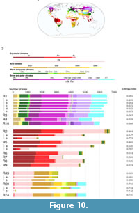the repartition of the sites in our dataset among the Köppen climate subclasses as a map, as well as the distribution of the support of the redescriptions over those subclasses as histograms. For each redescription, the histogram shows the number of sites from each subclass that belongs to its support. The legend, between the map and the histograms, indicates the total number of sites in each subclass grouped by class, with bars at the same scale as the histograms. Variants are listed below the main redescription they are associated with and are depicted with narrower histograms.

Note that overall this analysis is not aimed at finding redescriptions that match the Köppen climate subclasses one-to-one, but rather defining new classes driven by the match between traits and climate. Yet here, for comparison and general interest, we evaluate the match between a redescription’s support and the Köppen climate subclasses using the entropy measure. For a given redescription R, we consider the random variables X and Y to represent the membership of sites in the support of R and in a Köppen climate subclass, respectively. Letting s denote a site, we have X=1 if and only if s∈ supp(R), and X=0 otherwise. On the other hand, Y=k_i where k_i ∈K denotes the Köppen subclass to which the site belongs. Intuitively, the entropy of X, H(X), represents the amount of information that is contained in the variable X, while the entropy of X conditioned on Y, H(X|Y), represents the amount of additional information contained in X when Y is known. Hence, we take H(X|Y)/H(X) as a measure of the ratio of information contained in X that cannot be determined from Y.

A perfect match means that there exists a subset of Köppen subclasses such that a site belongs to the support of the redescription if and only if it belongs to one of the subclasses in the subset. In that case, the support can be entirely determined from the Köppen subclasses, we have H(X|Y)=0 and H(X|Y)/H(X)=0. On the other hand, if the match is very poor, knowing the subclasses does not bring any information about membership in the support, then H(X|Y) will be close to H(X) so that H(X|Y)/H(X)≈1. In short, H(X|Y)/H(X) will take value in the range [0,1], with redescriptions whose support matches the Köppen subclasses associated to smaller values.

We show the corresponding value of the entropy ratio, H(X|Y)/H(X), next to each redescription in Figure 10. We observe that the match between support and climate subclasses is best among redescriptions in the first group, especially R3 and R1, as well as the latter’s variants R1a and R1b, which have entropy ratios at or near 0.283. The match between the climate subclasses and the support of redescriptions from the second and third groups is somewhat worse, with ratios typically around 0.5 and 0.7, respectively. Again, our goal is not to find a perfect match between our redescriptions and the Köppen system, but this is clearly helpful when trying to interpret the obtained redescriptions. We now look in turn at each group more closely.

The support of redescriptions within the boreal-temperate moist group (R1, R3, R4, R10 and variants) belongs mainly to Köppen snow subclasses (class D), in part to Köppen warm temperate subclasses (class C), as well as to Köppen polar subclasses (class E) in North-East Asia and on the Tibetan plateau. Indeed, most of the snow subclasses (class E) and the humid subclasses (class C) of the warm temperate areas are covered by redescriptions from our first group and are not covered by our other two groups. The Tibetan plateau constitutes an exception to this repartition, as it also appears in redescriptions from the tropical-subtropical dry zone. Comparing Figure 10 and Figure 6 reveals that the query of dental traits in these redescriptions tends to capture some dry climate regions compared to the query of climate variables which limits the region in the temperate-cold humid climate.

Redescriptions within the tropical moist group (R2, R5–R9 and variants) consistently cover equatorial Köppen subclasses (class A) in South America, Africa and Indonesia-Malaysia regions (cf. Figure 10 and Figure 6). However, the tropical climate in India, South-East Asia and East Africa is not covered by these redescriptions. The inconsistencies between the dental traits and climate queries in these redescriptions mainly occur in South-East Asia, which only satisfies the dental traits queries, and East Africa, which only satisfies the climate queries. This suggests that the association between dental traits and climate in these regions is distinct from other tropical climate regions.

Redescriptions from the tropical-subtropical dry group (R43, R69, R74 and variants) mainly cover arid Köppen subclasses (class B) and seasonal dry climate types in tropical and subtropical regions (Aw, Cwa and Cwb) of India and East Africa, as expected from the formulation of the queries. As discussed earlier, redescriptions R69, R69a and R74 from this group cover the Tibetan plateau, an area classified within the polar class of the Köppen system (class E) but which also fits the pattern of seasonality captured by those redescriptions.

We observe that southern China and South-East Asia are not covered by the redescriptions reported in this study. This brings into focus the uniqueness of these regions in their dental traits-climate association. Indeed, while the climate types of these regions (especially Aw and Cwa) are similar to other tropical regions covered by our redescriptions, their dental traits typically follow more temperate-like patterns. In particular, these regions accommodate a relatively large share of brachydont species and a relatively high percentage of species with obtuse lophs, as can be seen from the trait maps in Figure 5. The summer monsoon in these regions may be attractive for immigrants from the temperate zone that enjoy the southern comfort. At the same time, due to a strong influence of Asian winter monsoon in these regions, winters are usually colder and drier than in other tropical areas. This may cause defoliation of trees in winter, and thus favor more temperate-like dental traits of the fauna that can help them to survive the harsh winter. Therefore, redescriptions capturing the association between climate and dental traits in this area do not generalize worldwide. Additionally, a large part of southern China is characterized by a warm temperate fully humid climate (Cfa), which is rather specific to that area (cf. Figure 10). For this reason, climate queries characterizing this region must either have very little overlap with other regions, or cover a very broad range of values. This specificity of the southern China climate is another probable reason for the lack of coverage by the top redescriptions of this area.

CONCLUSION

Redescription mining provides a means to discover associations between two sets of variables characterizing entities, in our case geographic sites. In this study, dental traits of large herbivorous mammals are used to characterize and find associations between the biotic environment and climatic conditions, characterized by temperature and precipitation variables. The resulting redescriptions can be considered as computational biomes identified in a data-driven way. We have compared the resulting redescriptions with the Köppen climate classification, and found a consistent match in support. The difference between climate classes and our approach is that the Köppen climate classification is defined in terms of climate only, whereas our redescriptions define zones by combining climate and species trait distributions.

Our analysis distinguishes three global zones, which we refer to as the boreal-temperate moist zone, the tropical moist zone and the tropical-subtropical dry zone. The boreal-temperate moist zone is mainly characterized by seasonal cold temperatures, a lack of hypsodonty and a high share of species with obtuse lophs. The tropical moist zone is mainly characterized by high temperatures, high isothermality, abundant precipitation and a high share of species with acute rather than obtuse lophs. Finally, the tropical-subtropical dry zone is mainly characterized by a high seasonality of temperatures and precipitation, as well as high hypsodonty and horizodonty. We find that the dental trait signature of African moist forests is quite different from the signature of climatically similar sites in North America and Asia. The share of high hypsodont species is notably high in Africa, while it is quite low in the modern day in North America and Asia, which may be partially due to severe anthropogenic effects in both these areas. In terms of climate and dental signatures, the African seasonal tropics share a lot of similarities with Central-South Asian sites. Interestingly, the Tibetan plateau is covered both by redescriptions from the tropical-subtropical dry group and by redescriptions from the boreal-temperate moist group, suggesting a combination of features from both zones in its dental traits and climate. This is different from common experience-based biome/climate classifications, which simply regard the Tibetan Plateau as a cold tundra biome/climate. On the other hand, southern China and South-East Asia are not covered by any of the redescriptions reported in this study, which suggests that the association between dental traits and climate in those areas is unique. Dental traits in China are similar to those of temperate zones, while the climate is most similar to that of the tropical zones covered by our redescriptions. The fact that the climate of this region, classified as Cfa in the Köppen system, is encountered only in few other locations worldwide and is hence fairly specific, further explains this lack of coverage.

Our study is aimed at finding associations between dental traits and climate. The resulting redescriptions specify these relationships, how strongly they hold and where they hold geographically. While mechanically simple, applying the redescriptions to the past requires us to carefully consider how to systematically evaluate the ability of the patterns to generalize to data coming from different sources and how to reconcile the diverging projections that may arise from different redescriptions. Most of palaeontology is, and has always been, ultimately based on understanding the modern world. Since Cuvier, teeth have figured bigly in this. Our study is primarily a contribution to a better understanding of functional relationships of teeth as an interface between animals and their edible environment.

ACKNOWLEDGMENTS

We thank M. Lawing and J.T. Eronen for consultations about species distribution data. The work of HT is supported by Land-ATmosphere Interactions in Cold Environments (LATICE), which is a strategic research area funded by the Faculty of Mathematics and Natural Sciences at the University of Oslo. MF and IZ acknowledge funding from the Academy of Finland (ECHOES project). This is a contribution from the Valio Armas Korvenkontio Unit of Dental Anatomy in Relation to Evolutionary Theory.

REFERENCES

Barr, W.A. 2017. Bovid locomotor functional trait distributions reflect land cover and annual precipitation in sub-Saharan Africa. Evolutionary Ecology Research, 18:253-269.

Brown, A.M., Warton, D.I., Andrew, N.R., Binns, M., Cassis, G., and Gibb, H. 2014. The fourth-corner solution—using predictive models to understand how species traits interact with the environment. Methods in Ecology and Evolution, 5(4):344-352. https://doi.org/10.1111/2041-210X.12163

Cleveland, C.C., Townsend, A.R., Taylor, P., Alvarez-Clare, S., Bustamante, M.M.C., Chuyong, G., Dobrowski, S.Z., Grierson, P., Harms, K. E., Houlton, B.Z., Marklein, A., Parton, W., Porder, S., Reed, S.C., Sierra, C.A., Silver, W.L., Tanner, E.V.J., and Wieder, W.R. 2011. Relationships among net primary productivity, nutrients and climate in tropical rain forest: A pan-tropical analysis. Ecology Letters, 14(9):939-947. https://doi.org/10.1111/j.1461-0248.2011.01658.x

Dominy, N.J., Lucas, P.W., and Wright, S.J. 2003. Mechanics and chemistry of rain forest leaves: Canopy and understorey compared. Journal of Experimental Botany, 54(390):2007-2014. https://doi.org/10.1093/jxb/erg224

Elith, J. and Leathwick, J.R. 2009. Species distribution models: Ecological explanation and prediction across space and time. Annual Review of Ecology, Evolution, and Systematics, 40(1):677-697. https://doi.org/10.1146/annurev.ecolsys.110308.120159

Eronen, J., Mirzaie Ataabadi, M., Micheels, A., Karme, A., Bernor, R., and Fortelius, M. 2009. Distribution history and climatic controls of the late Miocene Pikermian chronofauna. Proceedings of the National Academy of Sciences, 106(29):11867-11871. https://doi.org/10.1073/pnas.0902598106

Eronen, J., Puolamäki, K., Liu, L., Lintulaakso, K., Damuth, J., Janis, C., and Fortelius, M. 2010a. Precipitation and large herbivorous mammals, part I: Estimates from present-day communities. Evolutionary Ecology Research, 12(2):217-233.

Eronen, J., Puolamäki, K., Liu, L., Lintulaakso, K., Damuth, J., Janis, C., and Fortelius, M. 2010b. Precipitation and large herbivorous mammals, part II: Application to fossil data. Evolutionary Ecology Research, 12(2):235-248.

Eronen, J.T., Polly, P.D., Fred, M., Damuth, J., Frank, D.C., Mosbrugger, V., Scheidegger, C., Stenseth, N.C., and Fortelius, M. 2010c. Ecometrics: The traits that bind the past and present together. Integrative Zoology, 5(2):88-101. https://doi.org/10.1111/j.1749-4877.2010.00192.x

Food and Agriculture Organization of the United Nation. 1989. Arid Zone Forestry: A Guide for Field Technicians. FAO Forestry, Italy.

Fortelius, M. 1981. Functional aspects of occlusal cheek-tooth morphology in hypsodont non-ruminant ungulates, p. 153-162. In Martinell, J. (ed.), International Symposium on Concept and Method in Paleontology: Contributed Papers . Departament de Paleontologia, Universitat de Barcelona, Barcelona, Spain.

Fortelius, M., Eronen, J., Jernvall, J., Liu, L., Pushkina, D., Rinne, J., Tesakov, A., Vislobokova, I., Zhang, Z., and Zhou, L. 2002. Fossil mammals resolve regional patterns of Eurasian climate change over 20 million years. Evolutionary Ecology Research, 4(7):1005-1016.

Fortelius, M., Zliobaite, I., Kaya, F., Bibi, F., Bobe, R., Leakey, L., Leakey, M., Patterson, D., Rannikko, J., and Werdelin, L. 2016. An ecometric analysis of the fossil mammal record of the Turkana basin. Philosophical Transactions of the Royal Society B: Biological Sciences, 371(1698):1–13. https://doi.org/10.1098/rstb.2015.0232

Galbrun, E. and Miettinen, P. 2012. From black and white to full color: Extending redescription mining outside the Boolean world. Statistical Analysis and Data Mining, 5(4):284–303. https://doi.org/10.1002/sam.11145

Galbrun, E. and Miettinen, P. 2014. Interactive redescription mining, p. 1079–1082. In Dyreson, C.E., Li, F., Özsu, M.T. (eds.), Proceedings of the 20th ACM SIGMOD International Conference on Management of Data (SIGMOD’14) . ACM, New York, USA. https://doi.org/10.1145/2588555.2594520

Galbrun, E. and Miettinen, P. 2016. Analysing political opinions using redescription mining, p. 422-427. In Domeniconi, C., Gullo, F., Bonchi, F., Domingo-Ferrer, J., Baeza-Yates, R., Zhou, Z.H., Wu, X. (eds.), IEEE International Conference on Data Mining Workshops . Conference Publishing Services, IEE, USA. https://doi.org/10.1109/ICDMW.2016.0066

Gallo, A., Miettinen, P., and Mannila, H. 2008. Finding subgroups having several descriptions: Algorithms for redescription mining, p. 334-345. In Apte, C., Park, H., Wang, K., and Zaki, M.J. (eds.), Proceedings of the 8th SIAM International Conference on Data Mining (SDM’08) . SIAM, USA. https://doi.org/10.1137/1.9781611972788.30

Hannisdal, B., Haaga, K.A., Reitan, T., Diego, D., and Liow, L. 2017. Common species link global ecosystems to climate change: Dynamical evidence in the planktonic fossil record. Proceedings of the Royal Society of London B: Biological Sciences, 284:20170722. https://doi.org/10.1098/rspb.2017.0722

Heywood, J. 2010. Explaining patterns in modern ruminant diversity: Contingency or constraint? Biological Journal of the Linnean Society, 99:657-672. https://doi.org/10.1111/j.1095-8312.2010.01436.x

Jernvall, J. 1995. Mammalian molar cusp patterns: Developmental mechanisms of diversity. Acta Zoologica Fennica, 198:1-61.

Jernvall, J. and Fortelius, M. 2002. Common mammals drive the evolutionary increase of hypsodonty in the Neogene. Nature, 417:538-540. https://doi.org/10.1038/417538a

Kaiser, T.M., Fickel, J., Streich, W.J., Hummel, J., and Clauss, M. 2010. Enamel ridge alignment in upper molars of ruminants in relation to their natural diet. Journal of Zoology, 281(1):12-25. https://doi.org/10.1111/j.1469-7998.2009.00674.x

Kaiser, T.M., Muller, D.W.H., Fortelius, M., Schultz, E., Codron, D., and Clauss, M. 2013. Hypsodonty and tooth facet development in relation to diet and habitat in herbivorous ungulates: Implications for understanding tooth wear. Mammal Review, 43:34-46. https://doi.org/10.1111/j.1365-2907.2011.00203.x

Kay, R. and Hiiemae, K. 1974. Jaw movement and tooth use in recent and fossil primates. American Journal of Physical Anthropology, 40:227-256. https://doi.org/10.1002/ajpa.1330400210

Kottek, M., Grieser, J., Beck, C., Rudolf, B., and Rubel, F. 2006. World map of the Köppen-Geiger climate classification updated. Meteorologische Zeitschrift, 15(3):259-263. https://doi.org/10.1127/0941-2948/2006/0130

Lawing, A.M., Eronen, J.T., Blois, J.L., Graham, C.H., and Polly, P.D. 2016. Community functional trait composition at the continental scale: The effects of non-ecological processes. Ecography, 39:1-13. https://doi.org/10.1111/ecog.01986

Lawing, A. M., Head, J.J., and Polly, P.D. 2012. The ecology of morphology: The ecometrics of locomotion and macroenvironment in North American snakes, p. 117-146. In Louys, J. (ed.), Paleontology in Ecology and Conservation, Earth System Sciences . Springer Berlin Heidelberg. https://doi.org/10.1007/978-3-642-25038-5_7

Legendre, P. and Legendre, F. 2012. Numerical Ecology . Elsevier, The Netherlands.

Levering, D., Hopkins, S., and Davis, E. 2017. Increasing locomotor efficiency among North American ungulates across the Oligocene-Miocene boundary. Palaeogeography, Palaeoclimatology, Palaeoecology, 466(Supplement C):279-286. https://doi.org/10.1016/j.palaeo.2016.11.036

Lieth, H. 1975. Modelling the primary productivity of the world, p. 237-263. In Lieth, H. and Whittaker, R.H. (eds.), Primary Productivity of the Biosphere . Springer, New York. https://doi.org/10.1007/978-3-642-80913-2_12

Liu, L., Puolamäki, K., Eronen, J.T., Mirzaie Ataabadi, M., Hernesniemi, E., and Fortelius, M. 2012. Dental functional traits of mammals resolve productivity in terrestrial ecosystems past and present. Proceedings of the Royal Society B: Biological Sciences, 279:2793-2799. https://doi.org/10.1098/rspb.2012.0211

Madden, R.H. 2014. Hypsodonty in Mammals: Evolution, Geomorphology, and the Role of Earth Surface Processes . Cambridge University Press, Cambridge, UK.

McGuire, J.L. and Davis, E.B. 2014. Conservation paleobiogeography: The past, present and future of species distributions. Ecography, 37:1092-1094. https://doi.org/10.1111/ecog.01337

Melillo, J.M., McGuire, A.D., Kicklighter, D.W., Moore, B., Vorosmarty, C.J., and Schloss, A.L. 1993. Global climate change and terrestrial net primary production. Nature, 363:234-240. http://doi.org/10.1038/363234a0

Meloro, C. and Kovarovic, K. 2013. Spatial and ecometric analyses of the Plio-Pleistocene large mammal communities of the Italian peninsula. Journal of Biogeography, 40:1451-1462. https://doi.org/10.1111/jbi.12113

Polly, P.D. and Head, J.J. 2015. Measuring earth-life transitions: Ecometric analysis of functional traits from late Cenozoic vertebrates. The Paleontological Society Papers, 21:21-46. 

Popowics, T.E. and Fortelius, M. 1997. On the cutting edge: Tooth blade sharpness in herbivorous and faunivorous mammals. Annales Zoologici Fennici, 34(2):73-88.

Ramakrishnan, N., Kumar, D., Mishra, B., Potts, M., and Helm, R.F. 2004. Turning CARTwheels: An alternating algorithm for mining redescriptions, p. 266-275. In Gehrke, J. and DuMouchel, W. (eds.), Proceedings of the 10th ACM SIGKDD International Conference on Knowledge Discovery and Data Mining (KDD’04) . ACM, New York, USA. https://doi.org/10.1145/1014052.1014083

Reed, K. 2013. Multiproxy paleoecology: Reconstructing evolutionary context in paleoanthropology. In Begun, R.D. (ed.), A Companion to Paleoanthropology, p. 204-225. Wiley-Blackwell, Oxford. https://doi.org/10.1002/9781118332344.ch11

Saarinen, J. 2015. Ecometrics of Large Herbivorous Land Mammals in Relation to Climatic and Environmental Changes During the Pleistocene . PhD thesis, Department of Geosciences and Geography, University of Helsinki. http://urn.fi/URN:ISBN:978-952-10-9468-2

Schnitzler, J., Theis, C., Polly, P.D., and Eronen, J.T. 2017. Fossils matter—understanding modes and rates of trait evolution in Musteloidea (Carnivora). Evolutionary Ecology Research, 18:187–200.

Strömberg, C.A. 2002. The origin and spread of grass-dominated ecosystems in the late Tertiary of North America: Preliminary results concerning the evolution of hypsodonty. Palaeogeography, Palaeoclimatology, Palaeoecology, 177(1):59-75. https://doi.org/10.1016/S0031-0182(01)00352-2

Strömberg, C.A., Dunn, R.E., Madden, R.H., Kohn, M.J., and Carlini, A.A. 2013. Decoupling the spread of grasslands from the evolution of grazer-type herbivores in South America. Nature Communications, 4:1478. https://doi.org/10.1038/ncomms2508

Stuart, A.J., Kosintsev, P.A., Higham, T.F.G., and Lister, A.M. 2004. Pleistocene to Holocene extinction dynamics in giant deer and woolly mammoth. Nature, 431:684-689. https://doi.org/10.1038/nature02890

Sukselainen, L., Fortelius, M., and Harrison, T. 2015. Co-occurrence of pliopithecoid and hominoid primates in the fossil record: An ecometric analysis. Journal of Human Evolution, 84:25-41.

Thenius, E. 1989. Zähne und Gebiß der Säugetiere. In Niethammer, J., Schliemann, H., and Starck, D. (eds.), Handbook of Zoology, volume VIII, Mammalia, part 56 . Walter de Gruyter, Berlin.

Traiser, C., Klotz, S., Uhl, D., and Mosbrugger, V. 2005. Environmental signals from leaves—a physiognomic analysis of European vegetation. New Phytologist, 166(2):465–484. https://doi.org/10.1111/j.1469-8137.2005.01316.x

Ungar, P. S. 2014. Dental allometry in mammals: A retrospective. Annales Zoologici Fennici, 51:177-187. https://doi.org/10.5735/086.051.0218

Wang, P.X., Wang, B., Cheng, H., Fasullo, J., Guo, Z.T., Kiefer, T., and Liu, Z.Y. 2014. The global monsoon across timescales: Coherent variability of regional monsoons. Climate of the Past, 10:2007-2052. https://doi.org/10.5194/cp-10-2007-2014

Wolfe, J.A. 1995. Paleoclimatic estimates from Tertiary leaf assemblages. Annual Review of Earth and Planetary Sciences, 23:119-142. https://doi.org/10.1146/annurev.ea.23.050195.001003

Zinchenko, T., Galbrun, E., and Miettinen, P. 2015. Mining predictive redescriptions with trees, p. 1672-1675. In Cui, P., Dy, J., Aggarwal, C., Zhou, Z.H., Tuzhilin, A., Xiong, H., and Wu, X. (eds.), IEEE International Conference on Data Mining Workshops, IEEE Conference Publishing Services, USA. https://doi.org/10.1109/ICDMW.2015.123

Zliobaite, I., Rinne, J., Toth, A., Mechenich, M., Liu, L.P., Behrensmeyer, A.K., and Fortelius, M. 2016. Herbivore teeth predict climatic limits in Kenyan ecosystems. Proceedings of the National Academy of Sciences, 113(45):12751-12756. https://doi.org/10.1073/pnas.1609409113