Estimating spirals

Refined methods for estimating spirals and spiral deviations

Anthony E. Aldridge

Article number: 23(2):a41
https://doi.org/10.26879/1071
Copyright Paleontological Society, August 2020

Author biography
Plain-language and multi-lingual abstracts
PDF version

Submission:  18 February 2020. Acceptance: 10 August 2020.

ABSTRACT

Logarithmic spirals are near-perfect fits to the outlines of many accretionary structures. Spiral fitting has recently proved to be efficient at revealing shape changes, and growth periodicities important to taxonomic and paleoclimatic studies. However, the fitting lacks guidelines for choosing the type, or even a best spiral for an outline. Described here is a family of 12 logarithmic spirals that represent many types of accretion. A simple logarithmic spiral has one constant expansion rate relative to the angle turned about an axis. Increasing complexity leads to 11 more logarithmic spirals: three are piecewise logarithmic spirals, three are log-polynomial spirals, a pair combine logarithmic and log-polynomial spirals, then lastly, three are spirals that feature a transition between logarithmic segments. The supplementary R package logspiral generates and fits all 12 spirals, and includes a comprehensive catalogue of examples.

Comparing an actual accretionary outline to spirals in the catalogue highlights all nearest matches, ranked in order of a similarity ratio. Fitting nearest spirals to the outline helps choose the best spiral and its associated spiral deviations. Heuristics continue to be both quick and reliable for a final choice of spiral. The best spiral fit for an outline often produces a deviation pattern that is surprisingly consistent with all nearest spirals. The immediate value of other than a simple logarithmic spiral lies in the detection of otherwise hard to see breakpoints and other phase changes in growth that affect overall shape. Including a phase change, or changes in a spiral fit, then reveals any lurking cycles or periodicities in the growth. These periodicities as spiral deviations are considered to represent annual and seasonal growth.

Anthony E. Aldridge. PO Box 7, Wakefield, New Zealand 7052. tony@southnet.co.nz

Keywords: accretion; logarithmic; breakpoint; bent cable; periodicity; R package

Aldridge, Anthony E. 2020. Refined methods for estimating spirals and spiral deviations. Palaeontologia Electronica, 23(2):a41. https://doi.org/10.26879/1071
palaeo-electronica.org/content/2020/3135-estimating-spirals

Copyright: August 2020 Paleontological Society.
This is an open access article distributed under the terms of Attribution-NonCommercial-ShareAlike 4.0 International (CC BY-NC-SA 4.0), which permits users to copy and redistribute the material in any medium or format, provided it is not used for commercial purposes and the original author and source are credited, with indications if any changes are made.
creativecommons.org/licenses/by-nc-sa/4.0/

INTRODUCTION

Logarithmic spirals are a close fit to the accretionary outlines of many forms of growth (Hammer, 2016). However, close does not mean a perfect match to every point on an outline. The difference between a point of growth and the fitted spiral is termed a spiral deviation, or a shell spiral deviation (SSD) in the case of shell growth (Pérez-Huerta et al., 2014, Clark et al., 2016).

When a spiral fit practically matches actual growth, the SSDs invariably exhibit periodicities that can be interpreted as reflecting plausible ontogenetic ages for both living and fossil brachiopods (Aldridge and Gaspard, 2011; Pérez-Huerta et al., 2014; Clark et al., 2015; Gaspard et al., 2018). Age and growth rate estimates are vital for the study of life history, population dynamics, and climate (see Clark et al., 2015, and references therein).

As an outline, accretionary growth follows a trajectory from a given starting point. The outline is digitized as a series of coordinate points (i.e., sequential pairs of horizontal and vertical values for a 2D image). Points may or may not be equally spaced along an outline, if not, they can be later equally spaced or smoothed depending of the study objectives. Clark et al. (2015) have examples with code for digitizing and displaying outlines. This study builds on what is described in Clark et al. (2015).

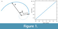Choice of spiral begins with the simplest. That is, a spiral with parameters analogous to a straight line (intercept and slope), using the logarithm of radius (log-radius) from an axis, and the angle turned as variables (Figure 1A). The intercept is the initial log-radius from the spiral axis to the spiral (zero angle turned), and the slope is a constant ratio of log-radius to angle turned (Figure 1B). The units of slope are usually quoted in terms of a whorl expansion rate, which on a natural logarithmic scale is the ratio of two radii after one full revolution of growth multiplied by 2π (Raup, 1966; McGhee, 1980). However, brachiopods and many molluscs exhibit well under a full revolution of growth so a whorl expansion rate is not easy to interpret on an actual shell. Alternatively, the slope can be converted as a constant angle between the spiral and a radius vector for a simple logarithmic spiral (Hammer, 2016, figure 9.2). The tangent vector with this angle is also the direction of growth, which itself can be decomposed into anterior and vertical components (Rudwick, 1959). Spiral angle is the choice here for describing the expansion of a logarithmic spiral. Inverting the slope then taking the inverse or arc tangent produces the spiral angle in radian units, which multiplication by 180/π converts radians to degrees. A zero-degree spiral angle has a flat outline, whereas a 90-degree spiral angle has a circular outline. Spiral angle is thus a useful measure of outline inflation, but spiral angle must not be confused with the angle turned about the spiral axis. When estimating the spiral angle a complication arises, because the spiral axis is unknown so we also need to estimate the location of the spiral axis (two values for an outline in 2D). Fitting the simplest spiral then becomes iterative and requires nonlinear least squares to simultaneously estimate four values: start log-radius, spiral angle and two values for axis location (Kimberley, 1989; Aldridge, 1998).

While the simplest spiral provides a close fit to most accretionary outlines, spiral deviations are key to whether a suitable spiral form has been chosen. Sometimes, having a more complex spiral results in only minor changes to the deviation pattern, so age estimates remain the same, and the simple spiral is retained (Clark et al., 2015, figure 9). Other times, there is a dramatic and clear shape to the spiral deviations that demands the use of a more complex spiral to fit a growth outline (Aldridge, 1999, figure 2). Clark et al. (2015) conclude that a “refinement in methodology” is needed for fitting spirals and the choice of spiral.

We improve spiral fitting by first describing a family of spirals suitable for a wide range of accretionary outlines. The open source software R (R Core Team, 2020) with the package logspiral is available for generating and fitting these spirals (Appendix 1 has instructions for downloading and installing Supplemental Material  logspiral). The best spiral fit to an outline confirms the presence, or not, of any major disturbance or break that changes shape during growth. Such changes are practically impossible to see ‘by eye’ when a continuous, smooth curve appears to dominate an outline. Fitting a spiral on a few individuals aims to elicit knowledge of any major shape changes in a species or population. In addition, extracting spiral deviations exposes any lurking periodicities or cycles in growth. The remainder of this study shows how to use logspiral to find spirals nearest to an actual outline, then how to choose a best fitting spiral along with its spiral deviations.

METHODS AND RESULTS

Family of Spirals

Spirals classify according to their relationship between the logarithm of the radius (log-radius) and the increasing angle about a spiral axis. The relationship of log-radius with turning angle allows spirals to be developed in a similar way to standard polynomial and segmented regression models (e.g., Draper and Smith, 1981). Segmented models with one or more connected spirals have proved useful in describing outline shape, and indicated the presence of a phase change in accretionary growth particularly for adult brachiopods (Aldridge, 2011; Pérez-Huerta et al., 2014; Gaspard et al., 2018). The previous restriction of having only abrupt change or breakpoint in a spiral is now relaxed to include a transition between different spiral episodes on the same outline.

In keeping with standard regression models, classification begins with the simplest possible logarithmic spiral. A single logarithmic spiral with constant expansion ratio (slope) of log-radius to angle turned is called a L1 spiral (Figure 1B). Episodes of spirals, with each episode having a different ratio or spiral angle on the same outline, were first described by Aldridge (1999). Spirals with up to four episodes of growth are now called L2, L3, and L4 spirals (Figure 2, top panel). While the L3 and L4 spirals might seem unlikely to represent actual growth, their value mostly lies in approximating the more complex spirals (see Discussion below).

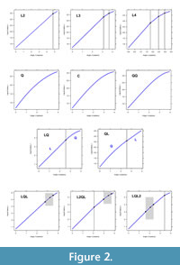A continuous, second order change in the expansion rate was initially described by adding a quadratic term to the simple logarithmic spiral (McGhee, 1980). As with polynomial regression models, there can be third and fourth order changes in the expansion rate leading to the definition of log-cubic and log-quartic spirals. In terms of a log-polynomial relationship between log-radius and angle about a spiral axis the classification includes the log-quadratic (Q), log-cubic (C), and log-quartic (QQ) spirals (Figure 2, second row of graphs).

The next extension concatenates the simple logarithmic (L1) and log-quadratic (Q) as one spiral shape. Having log-quadratic at either the earlier or the latter part of a simple logarithmic spiral leads, respectively, to the log-quadratic-linear (QL), and the log-linear-quadratic (LQ) spirals (Figure 2, third row). Allowing a transition between two simple logarithmic spirals describes a bent cable (Chiu et al., 2006) as a spiral, and a generalized bent cable (Khan and Kar, 2018) as a spiral. (LQL, Figure 2, bottom left). While the bent cable forces this transition to be a quadratic shape, the generalized bent cable allows a fractional power to the transition (i.e., not the fixed 2.0 power of the quadratic). The bent cable then becomes a special case of the generalized bent cable so both are referred to here as a LQL spiral. Including another simple logarithmic segment at the start, or at the end of a bent cable leads to the logarithmic-bent cable and the bent cable-logarithmic spirals (L2QL and LQL2 see Figure 2, bottom row).

Abbreviating the names of spirals allows concise description when generating, cataloguing, comparing, and fitting spirals. Table 1 displays these abbreviations for quick reference, and Table 2 has a glossary of terms used. The supplementary R package logspiral contains all 12 spirals for both generating and fitting these spirals. There is nothing magic or necessarily complete about the number 12 for this family of spirals. The spirals in this family mirror what is done when extending linear regression models (e.g., Draper and Smith, 1981). More importantly, the spirals here are based on experience with fitting the growth of brachiopods and molluscs (e.g., Clarke et al., 2015; Aldridge, 2009), many of which appear as examples in the R package logspiral.

Matching an Outline to a Known Spiral

Examination of what doesn’t fit is standard practice with any model fitting to test adequacy and possible need for an alternative model (e.g., Draper and Smith, 1981). An adequate fit is one without any pattern to the deviations, while a non-random pattern can immediately suggest the form of a better fit. For example, in standard multiple regression an inverted U, or ‘∩’ shape to deviations suggests adding a quadratic or piecewise linear term to an independent variable (Draper and Smith, 1981). In contrast, spiral fitting is complicated by the underlying shape known to be curved with an axis to be estimated and the likely presence of growth periodicities. Unlike standard regression, the form of a better spiral fit is not visually straightforward to discern from the deviations of an L1 fit. For example, a log-piecewise logarithmic spiral (e.g., an L2 or an L3 spiral) often has deviations from an L1 fit with a distinctive ‘M’ rather than a ‘∩’ shape (Aldridge, 1999). Fitting an L1 spiral to very different spirals can have visually similar deviation patterns with only slight distortions in the ‘M’ shape. So subtle differences in the spiral deviation pattern differences do matter, depending on where and how much spirals change along an outline.

Blind or exhaustive searching for a better spiral depends on finding suitable starting values for the nonlinear algorithm, especially in the more complex models such as bent cable (e.g., Chiu et al 2006). Unless suitable starting values are input, the fitting can fail to converge, or end up on a local, and not the global optimum. An investigator can be left puzzling over whether or not a better spiral fit is possible. Could the overall pattern (e.g., the ‘M’ shape) of deviations help find a better fit? Would the finer detail (e.g., distortion in the ‘M’ shape) help? Or, perhaps a combination of overall pattern and detail would indicate a better spiral to fit? Described below is an analysis of the deviations from an L1 fit that combines their overall pattern using Fourier decomposition with their more local detail using wavelet decomposition. Candidate spirals for a better fit are chosen from a list that also suggests potential starting values. The list provided here is termed a catalogue and is also described along with its use.

First, a simple logarithmic spiral (L1) is fitted to an actual outline. The R package logspiral uses the base R function nls (nonlinear least squares) with the default Gauss-Newton algorithm. The iterative algorithm requires starting values, which logspiral supplies to cope with many outlines. There is also the option of user starting values, most often for a guess at the initial spiral axis location (this can be done interactively on a graphics device with logspiral). The initial axis location should be inside the outline and near the start of growth (see Clark et al., 2015). The L1 fit works well on most spiral shapes. The only exceptions appear to be when there is little or no curvature at the beginning of growth, or where curvature at the end of growth exceeds that at the beginning (a workaround is to fit only the first part of an outline to estimate better starting values).

Next, the resulting spiral deviations are scaled so their range is 10 units, and the total distance of growth lies between zero and 100 units. Spiral deviations are also linearly interpolated to 1,024 values of equally spaced growth distance. The resulting pattern of deviations with increasing growth is then decomposed into spectra based on Fourier frequencies (Bloomfield, 2000), and wavelet scales (Percival and Walden, 2000). Fourier variances are estimated using the base R function fft (R Core Team, 2020), using the first 20 pairs of complex frequencies (absolute value, squared and divided by 1,024). The wavelet variances result from using the maximal overlap, discrete transform function wavMODWT of the R package wmtsa (Constantine and Percival, 2017). The default wavelet shape is the Daubechies least asymmetric filter with eight coefficients (Percival and Walden, 2000). Successive filter scaling is based on powers of two so the maximum number of wavelet variances is 10 (2 10 = 1024). In summary, the pattern of scaled spiral deviations from an L1 fit to an actual outline is saved as 30 features: the first 20 variances of the Fourier spectrum and the 10 variances of the wavelet spectrum.

The last stage compares the outline’s 30 features of L1 spiral deviations against a catalogue of 838 known spiral instances, each with their own L1 deviation features. The catalogue was generated by varying the spiral angle and the location of spiral change for spirals in the family. Changes of spiral were spaced at 25%, 50%, and 75% along a generated outline. Spiral angles ranged from 30 to 80 degrees. Each spiral had 200 outline points generated, then a single spiral (L1) is fitted to compute the 30 features of the spiral deviations as described above. The catalogue is a table of 838 rows where the first 13 columns are values used to generate each spiral, and the next 30 columns are the features of the deviations from an L1 fit to each spiral.

The symmetric ratio of Choi et al. (2008) is applied to estimate the similarity or closeness of an actual outline’s L1 features to each of the 838 spirals in the catalogue. This ratio represents a summation of differences between variance features of the outline to a known spiral, separately for the Fourier and the wavelet features. Wavelets are considered more sensitive to transient cycles than the overall cycles represented by frequencies of the Fourier spectrum (Percival and Walden, 2000). Hence, the wavelet-based symmetric ratios are called local, while the Fourier are called global. A zero-value ratio (logarithm of unity) means a perfect match of the outline to a known spiral. A larger, negative ratio value implies a less match to a catalogued spiral. Candidate spirals are ranked on the similarity ratio, and the nine nearest spirals are presented, according to the wavelet scalogram (local) and the Fourier spectrum (global) L1 deviation features.

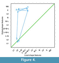
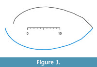As an example of outline matching we use the ventral valve of the brachiopod LR-FR1 in Pérez-Huerta et al. (2014, where figure 2A is a photograph of the sagittal section). Outlines of dorsal and ventral valves are reproduced with permission here as Figure 3 with 300 equally spaced points along the growth of each valve. This specimen is an adult of a species known to have a phase change in shape between juvenile and adult (Endo, 1987). Adult shells are more inflated or convex than juveniles. The outline data of LR-FR1 is in the R package logspiral, and the code to reproduce the ventral valve matching is in Appendix 1. Figure 4 shows the nine nearest spirals, ranked from one to nine. Closest on local features is the linear to bent cable spiral (L2QL) and on global features the log-quartic spiral (QQ). Both local and global features agree on a catalogue match with the abrupt change spiral, L2. So overall for this valve’s growth, there is evidence of a curved log-radius relationship to angle turned. Also, four spirals now need investigating in a ranked order of complexity: L2, L2QL, QQ, and C spirals.

Choosing a Spiral Fit

More than one type of spiral can be fitted to any given outline. Spiral fitting is more specialized than standard regression because in addition to the spiral shape parameters, every fit requires estimation of the spiral axis as a pair of Cartesian coordinates. An exhaustive search, fitting all 12 spirals to an outline may pose problems as the iterative, nonlinear method can fail from poor starting values or an inappropriate spiral being applied. Recommended here is to compare the outline’s L1 deviation features to a catalogue, then list nearest spirals to fit, and if necessary, use the list to find the realistic starting values for the nonlinear least squares algorithm.

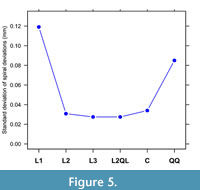Each spiral fit produces a sum of squared spiral deviations, which after dividing by the number of observations less spiral parameters and taking the square root becomes a residual standard deviation. The spiral with the least standard deviation is generally, but not always, the best spiral for a particular outline. A scree graph (Jolliffe, 2002) provides a visual method of comparing spiral fits. The example of the previous section has a scree graph that shows the L2 and L2QL spirals as having the least residual standard deviation (Figure 5). The L3 spiral was included as it was used to estimate another possible change that could be then input to fitting the L2QL spiral (see Appendix 1 for code). The most likely spiral shapes for this outline appear to be L2, L3, and L2QL. The log-quartic spiral (QQ) was excluded for being a poorer fit, and the log-cubic (C) was excluded because of unstable parameter estimates that changed markedly with slightly different starting values to the fit.

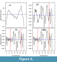Potential spiral candidates for an outline can also be compared by viewing their spiral deviation pattern with growth or arc length. For the ventral valve example, the L3 and L2QL spirals show very similar deviation patterns (Figure 6). This is explained by the L2QL spiral having a narrow transition zone, akin to being an abrupt change, so the L2QL spiral can be considered as equivalent to an L3 spiral for this valve’s growth. Final choice of spiral for the valve is between the L2 and L3 spiral. Adjusted for number of estimated parameters, both L2 and L3 have similar residual standard deviation. On the basis of being a simpler model, the L2 spiral is the final choice for accretionary growth in the LR-FR1 ventral valve.

When fitted spirals have similar sums of squared deviations and similar overall deviation patterns, other criteria can be applied. For example, an extreme deviation at, or very near, where spiral episodes abruptly change along an outline is evidence for choosing a spiral with a transition between episodes (logspiral gives a warning when this happens in a fit).

Another criterion considers how the variation in spiral deviations partition into low and higher Fourier frequencies. A dominant low frequency indicates a poor choice of spiral, often seen as the ‘M’ shape to spiral deviations when episodes have not been included in the fit (Figure 6, top left). A best choice fit is usually one that has the least low frequency variation and is dominated by a peak or peaks at moderate frequency (i.e., cyclic or periodic) components. The function doSpectrum in logspiral provides a quick visual guide of Fourier variances against frequency (as a wave number).

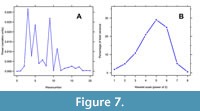The LR-FR1 ventral valve outline has a Fourier spectrum of L2 spiral deviations that show only noise or random variation in the first three wave numbers and after the 11 th wave number (Figure 7A). In between these wave numbers, there are several peaks (Figure 7A). The Fourier spectrum suggests that sinusoidal cycles at four frequencies (wave numbers 4, 5, 9, and 11) will explain the periodic component of L2 spiral deviations.

On the other hand, the wavelet scalogram has a maximum variance explained at the fifth scale interval (Figure 7B). At this 2 5 or 32 unit scale, periodicity explains 30% of total spiral deviation variation. The 300 equally spaced outline points in the LR-F1 ventral outline and the dominant wavelet scale provides an estimate of nine (300/32) cycles in the spiral deviations. Results from wavelet analysis of this valve are presented in Pérez-Huerta et al. (2014, figure 4) and provide an age of at least six years along with estimates of annual growth increments. Appendix 2 has recommended steps for choosing the best spiral and associated functions in the R package logspiral.

DISCUSSION

Coordinates of any digitized accretionary outline are viewed here as having four components of variation: the underlying shape that tracks growth, systematic change (i.e., major disturbances, phase changes, and cycles), then the biological and measurement noise. Here, the underlying shape can be any one of 12 logarithmic spirals, seven of which incorporate systematic change through connected or transitional spirals. All other variation is estimated from the spiral deviations. Cycles or periodicities are detected by applying wavelet and Fourier methods. Measurement and biological noise are not separated, but combine as the higher frequency components of spiral deviations. Because investigations usually begin without any knowledge of systematic changes or cycles in growth, the number of outline coordinates needs to be greater than 100 points per outline. For example, discerning transitional change, and the form of more than six growth cycles, the LR-F1 example used 300 equally spaced points along the ventral valve. In retrospect, 150 to 200 points would have sufficed to detect the cycles in LR-F1, but a cautionary approach here is to over rather than under sample an outline. However, there has to be a balance between the number of coordinate points possible, and the inherent precision in the image or specimen itself. For moderate size bivalves (e.g., between 10 and 100 mm), the digitized points may need precision of ± 0.1mm, or better.

A key assumption is that the spiral type contributes most of the variation in an outline. Finding the best spiral fit begins with an L1 fit then exploits the resulting deviation pattern to discern if there are any better spirals. While the L1 fit is often wrong for an outline, it rarely fails to produce parameter estimates. Steps toward a best spiral can be thought of as a ‘one wrong makes a right’, and particularly useful for any adult or well-developed accretionary structures. Juvenile forms may only have growth periodicities about an underlying L1 spiral. As one reviewer rightly commented, the log-piecewise, L4, spiral fit could also explain annual cycles in a four-year-old shell. This incorrect fitting is avoided by first noticing that cycles rather than a sharp ‘M’ or a distorted ‘M’ are often seen in the pattern of deviations from an L1 fit. Assuming annual cycles would be similar, another clue would be the gentle, rather than sharp decrease in a scree plot of standard deviations from each spiral fit. The choice between log-piecewise spirals and an L1 fit with cycles is most problematic when there are two, possibly annual, cycles without a strong ‘M’ deviation pattern. In this case, choice of a suitable spiral requires subject matter expertise such as knowing whether the outline is from a juvenile or from short-term growth.

Unknown is the impact of choosing the wrong spiral as a best fit. Checking an outline against a comprehensive catalogue of 838 instances goes some way to avoiding a bad spiral choice for an actual outline. Ranking and listing the nine nearest spirals to an outline is meant as a practical guide toward choosing a best spiral. The catalogue of generated spirals is based on a limited combinatorial set of parameter values, such as the location of a spiral change on an outline. So far when fitting accretionary growth only the L2 and the transitional bent cable spirals appear to be common. With the exception of the log-quartic spiral (included as an example in R package logspiral), none of the log-polynomial spirals have so far been found suitable for actual growth. It is expected that the catalogue will expand as more specimens are investigated.

As yet, there is no definitive statistical test for comparing one spiral to another. The spirals here are mostly not related or nested in a way that is conducive to ratios of test statistics. In addition, all outline points have strong auto correlation that inhibits easy estimation of inherent noise for any spiral. Ranking of nearest spirals from the catalogue is a novel approach to testing between spirals, which could be automated to incorporate computer-based learning methods (e.g., Efron and Hastie, 2016).

The nonlinear fitting of spirals is sensitive to the starting values for unknown parameters such as axis location and spiral angles. Even a slight perturbation from actual parameter values can cause the fitting to fail for spirals other than the simple logarithmic spiral (L1). Listing the nearest spirals (to a given outline) from a catalogue can be a quick and practical guide to suitable spirals and starting values. Another way is to use functions in logspiral to generate spirals on a trial and error basis to match a given outline. Alternatively, the L3 and L4 spirals and their change locations can be used to approximate log-polynomial and spirals with a bend between piecewise logarithmic sections on an outline. The spiral angles of L3 and L4 spirals are often suitable starting values for sections of spirals with a transition in their growth rates.

The immediate benefit of fitting other than the simple spiral (L1) is the detecting of important changes in specimen growth as it affects shape. Whether changes are abrupt or transitional offer clues as to the underlying causes and growth processes. The LR-F1 is an example in what may be common in many brachiopods. Taxonomic studies often describe overall shape through scatter plots of shell length, width and thickness. Less often do these studies have a complete size range (e.g., small shells can be winnowed from a population), or have sufficient specimens (e.g., few fossils at a site) to detect any change in shape through scatter plots or other multivariate methods. Fitting a suitable spiral on individual growth outlines can highlight any major shape change. That is, evidence of shape change can be predicted through fitting spirals to just a few specimens. Aldridge (2011, figure 5) shows for one extant brachiopod species that the L2 spiral fitting to seven adults provides the same detail on a shape breakpoint as does a scatter plot of shell length and thickness for 63 individuals. While spiral fitting reveals major changes in brachiopod shape, the causes remain arguable and still important to investigate. Aldridge (2011) summarizes these arguments with preference for stability and bonded substrate being the drivers for shape change in brachiopods.

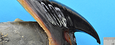
Another benefit of fitting is to expose any lurking cycles or periodicities in growth. The L2 spiral deviations of the LR-F1 example (Figure 6) have peaks and troughs that partially match stable isotopes in the shell, especially Magnesium, which has a known link to seawater temperature (Pérez-Huerta et al., 2014, Clark et al., 2016). Thus, shell spiral deviations have potential utility for the study of seasons and climate. Additionally, the number of peaks and troughs appear to be consistent with known age and growth rates, at least for some brachiopods (e.g., Aldridge and Gaspard, 2011, Gaspard et al., 2018). In contrast to the abrupt shape changes in brachiopods, there is evidence of transition spirals in non mineral squid beaks. Appendix 3 applies the refined spiral methods to the upper beak of one colossal squid for new results and hypotheses about the growth and age of this top predator, reported by Remeslo et al. (2019) as being enigmatic with access to complete specimens being rare.

In conclusion, the refined methods for spirals reported here are considered necessary when investigating the taxonomy or life history of any accretionary growth process.

ACKNOWLEDGEMENTS

We thank Professor D. Percival of Applied Physics Laboratory (University of Washington) for answering questions, and his website resources with slides, talks, and articles about wavelet analysis. We are grateful for Dr. R. Davies (Statistics Research Associates Ltd) who kindly supplied most of the Fourier spectrum function as S-plus code and the Museum of New Zealand Te Papa Tongarewa and B. Marshall for access to the colossal squid beak. Thanks also go to two referees and editors whose thorough critique and suggestions improved this manuscript.

REFERENCES

Aldridge, A.E. 1998. Brachiopod outline and the importance of the logarithmic spiral. Paleobiology, 24:215-226.

Aldridge, A.E. 1999. Brachiopod outline and episodic growth. Paleobiology, 25:471-482. https://doi.org/10.1017/s0094837300020339

Aldridge, A.E. 2009. Can beak shape help to research the life history of squid? New Zealand Journal of Marine and Freshwater Research, 43:1061-1067. https://doi.org/10.1080/00288330.2009.9626529

Aldridge, A.E. 2011. Ontogenetic discontinuities in brachiopod populations: their detection and significance. Memoirs of the Association of Australasian Paleontologists, 41:195-204

Aldridge, A.E. and Gaspard, D. 2011. Brachiopod life histories from spiral deviations in shell shape and microstructural signature - preliminary report. Memoirs of the Association of Australasian Paleontologists, 41:256-268.

Bloomfield, P. 2000. Fourier Analysis of Time Series: An Introduction, Second Edition. John Wiley and Sons, New York. https://doi.org/10.1002/0471722235

Chiu, G., Lockhart, R., and Routledge, R. 2006. Bent-Cable regression theory and applications. Journal of the American Statistical Association, 101:542-553. https://doi.org/10.1198/016214505000001177

Choi, H., Ombao, H., and Ray, B. 2008. Sequential change-point detection methods for nonstationary time series. Technometrics, 50:40-52. https://doi.org/10.1198/004017007000000434

Clark J., Aldridge, A., Reolid, M., Endo, K., and Pérez-Huerta, A. 2015. Application of shell spiral deviations methodology to fossil brachiopods. Palaeontologica Electronica, 18.3.54A:1-39. https://doi.org/10.26879/577
palaeo-electronica.org/content/2015/1189-brachiopod-spiral-deviations

Clark J., Pérez-Huerta, A., Gillikin, D., Aldridge, A., Reolid, M., and Endo, K. 2016. Determination of paleoseasonality of fossil brachiopods using shell spiral deviations and chemical proxies. Paleoworld, 25:662-674. https://doi.org/10.1016/j.palwor.2016.05.010

Constantine, W. and Percival, D.B. 2017. wmtsa: Wavelet Methods for Time Series Analysis. R package version 2.0-3. http://CRAN.R-project.org

Draper, N. and Smith, H. 1981. Applied Regression Analysis, Second Edition. John Wiley & Sons, New York. https://doi.org/10.1002/9781118625590

Efron, B. and Hastie, T., 2016. Computer Age Statistical Inference. Cambridge University Press, New York. https://doi.org/10.1017/CBO9781316576533

Endo, K. 1987. Life habit and relative growth of some Laqueid brachiopods from Japan. Transactions and Proceeding of the Palaeontological Society of Japan, 147:180-194. https://doi.org/10.14825/prpsj1951.1987.147_180

Gaspard D., Aldridge, A.E., Boudoumac, O., Fialind, M., Rividid, N., and Lécuyeref, C. 2018. Analysis of growth and form in Aerothyris kerguelenensis (rhynchonelliform brachiopod) - shell spiral deviations, microstructure, trace element contents and stable isotope ratios. Chemical Geology, 483:474-490. https://doi.org/10.1016/j.chemgeo.2018.03.018

Hammer, Ø. 2016. The Perfect Shape -Spiral Stories. Springer, Cham. https://doi.org/10.1007/978-3-319-47373-4

Jolliffe, I.T. 2002. Principal Component Analysis, Second Edition. Springer, New York.

Khan, S.A. and Kar, S.C. 2018. Generalized bent-cable methodology for changepoint data: a Bayesian approach. Journal of Applied Statistics, 45:1799-1822. https://doi.org/10.1080/02664763.2017.1391754

Kimberley, M.M. 1989. Fitting a logarithmic spiral to the shoreline of a headland-bay beach. Computers and Geosciences, 15:1089:1108. https://doi.org/10.1016/0098-3004(89)90121-0

McGhee, G.R.1980. Shell form in the biconvex articulate Brachiopoda: a geometric analysis. Paleobiology, 6:57-76. https://doi.org/10.1017/s0094837300012513

Percival, D.B. and Walden, A.T. 2000. Wavelet Methods for Time Series Analysis. Cambridge University Press, New York.

Pérez-Huerta, A., Aldridge, A.E., Endo, K., and Jeffries, T. E. 2014. Brachiopod shell spiral deviations (SSD): implications for trace element proxies. Chemical Geology, 374-375:13-24. https://doi.org/10.1016/j.chemgeo.2014.03.002

Raup, D.M. 1966. Geometric analysis of shell coiling: general problems. Journal of Paleontology, 40:1178-1190.

Remeslo, A., Yukhov, V., Bolstad, K., and Laptikhovsky, V. 2019. Distribution and biology of the colossal squid, Mesonychoteuthis hamiltoni: new data from depredation in toothfish fisheries and sperm whale contents. Deep Sea Research Part I: Oceanographic Research Papers, 147:121-127. https://doi.org/10.1016/j.dsr.2019.04.008

Rudwick, M.J.S. 1959. The growth and form of brachiopod shells. Geological Magazine, 96:1-24. https://doi.org/10.1017/s0016756800059173

R Core Team. 2020. R: A language and environment for statistical computing. R Foundation for Statistical Computing, Vienna, Austria. https://www.R-project.org/