

 BoneProfileR: The next step to quantify, model, and statistically compare bone section compactness profiles
Article number: 25.1.a12
https://doi.org/10.26879/1194
Copyright Paleontological Society, April 2022
Author biographies
Plain-language and multi-lingual abstracts
PDF version
Submission: 14 October 2021. Acceptance: 4 April 2022.
ABSTRACT
Bone sections have been widely used for over a century to assess life history traits of extant and extinct vertebrates, and they remain extremely useful. The characterization of their geometric and microanatomical properties forms the core of many descriptive and inferential studies. Bone compactness in particular has been associated with various attributes in individuals, such as habitat use or specific morphofunctional traits. A method implemented in software was published in 2003 to reduce the complexity of bone sections to facilitate quantitative analyses. We improve this method using better statistical tools (maximum likelihood and Bayesian analysis), a new function to model compactness, and we propose new enhanced software, BoneProfileR, as an R package, along with an online version for users unfamiliar with this language. Application of the new method to the femur of an extant hedgehog (Erinaceus europaeus) and a Permian temnospondyl (Eryops megacephalus) allows us to quantitatively and objectively describe the cross-sectional microanatomy of these two taxa.
Jordan Gônet. Centre de recherche en paléontologie - Paris, UMR 7207, Muséum national d’histoire naturelle, Sorbonne Université, Centre national de la recherche scientifique, 8 rue Buffon, CP 38, 75005 Paris, France. jordan.gonet@edu.mnhn.fr
Michel Laurin. Centre de recherche en paléontologie - Paris, UMR 7207, Muséum national d’histoire naturelle, Sorbonne Université, Centre national de la recherche scientifique, 8 rue Buffon, CP 38, 75005 Paris, France. michel.laurin@mnhn.fr
Marc Girondot. Laboratoire Ecologie, Systématique et Evolution, UMR 8079, Université Paris Saclay, AgroParisTech and CNRS, 91405 Orsay cedex, France. marc.girondot@universite-paris-saclay.fr
Keywords: bone section; bone compactness; model selection; paleobiology
Final citation: Gônet, Jordan, Laurin, Michel, and Girondot, Marc. 2022. BoneProfileR: The next step to quantify, model, and statistically compare bone section compactness profiles. Palaeontologia Electronica, 25(1):a12. https://doi.org/10.26879/1194
palaeo-electronica.org/content/2022/3590-bone-section-compactness-model
Copyright: April 2022 Paleontological Society.
This is an open access article distributed under the terms of Attribution-NonCommercial-ShareAlike 4.0 International (CC BY-NC-SA 4.0), which permits users to copy and redistribute the material in any medium or format, provided it is not used for commercial purposes and the original author and source are credited, with indications if any changes are made.
creativecommons.org/licenses/by-nc-sa/4.0/
INTRODUCTION
Bone cross-sections show many characteristics that have been used since the 1820s and 1830s to infer various properties of the individual or taxon from which they were prepared (Ricqlès 2021): life history traits (Amson et al. 2014), locomotor patterns (Houssaye et al. 2016), habitat (Jaquier and Scheyer 2017), metabolism, or growth rate (Faure-Brac and Cubo 2020; Chinsamy and Warburton 2021) are some examples. However, bone microstructure is very complex, and few objective, quantitative methods (other than very simple ones, like the cortico-diaphyseal index or the global compactness) were available to describe bone sections in a way that enables statistical inferences or comparisons (Castanet and Caetano 1995; Buffrénil and Francillon-Vieillot 2001).
In 2003, a computer program named Bone Profiler was produced to model bone tissue distribution in sections (Girondot and Laurin 2003). The main idea was to reduce bone section complexity to a limited number of variables that can be further compared using statistical tests. The development of software associated with this method was necessary to ensure reproducibility and precision of results. The original publication has been cited 129 times according to Google Scholar (as of September 15, 2021), which demonstrates its interest in ecology and paleobiology. The software was developed first in FutureBasic for MacOS and then converted into REALbasic to produce code for Windows, MacOSX and Linux systems. REALbasic was discontinued in 2006 and transformed into Xojo (Xojo, Inc.), but the original Bone Profiler code was no longer compatible with this compiler. This situation prevents adding new functionalities to the software and new enhancements of the original methodology. More recently, we were contacted by several researchers noting that the last available version of the software had stopped working on recent computers. They expressed concerns, because the method described in Girondot and Laurin (2003) has become a standard method in paleobiology, and it is important to continue to make it available for paleobiological and comparative studies. We produced a new enhanced version of the method and the software to fulfill this need. Below, we describe the method and software (new version is named BoneProfileR) with emphasis on the enhancement as compared to the original method and software (named Bone Profiler).
The method is applied to two taxa: the extant terrestrial mammal Erinaceus europaeus and the extinct amphibious temnospondyl Eryops megacephalus. Visually, they show microanatomical differences in cross-section that may be related to their respective lifestyles and possibly other factors. Erinaceus has a thick cortex and a well-defined medullary cavity, whereas Eryops has a thinner cortex and a medullary cavity invaded by cancellous bone. We use BoneProfileR to quantitatively and objectively describe these two sections.
SYSTEMS, METHODS AND ALGORITHMS
The standard procedure to analyze bone sections is the same as for the original 2003 version: 1) digitize a histological section or a drawing thereof; 2) open a bone section image; 3) locate the center of the bone section; 4) estimate bone compactness in concentric surfaces; 5) model the bone compactness using a mathematical function; and 6) compare bone compactness from various bone sections.
Bone Profiler was able to automatically handle all these steps, making the comparison easy and reproducible. The new version is developed as an R package available in CRAN (https://CRAN.R-project.org/package=BoneProfileR) and uses the same procedure. However, it is more convenient to use the statistical functions available in other R packages for step 6. A web-based version with a GUI (Graphical User Interface) has also been produced to help researchers unfamiliar with the R command line interface to use the method within the R package (http://134.158.74.46/BoneProfileR/).
Opening Images
Most standard graphic formats (JPEG, TIFF with or without Lempel-Ziv-Welch compression [lzw], BMP, PICT, PNG, GIF) can be read by the program using the function BP_OpenImage(). The TIFF image import can be done using the ijtiff package (Nolan and Padilla-Parra 2018) to handle special properties of some TIFF images generated by ImageJ (Rueden et al. 2017). After reading an image, the first step is to detect background (unmineralized) and foreground (mineralized) colors. This action can be done manually using BP_ChooseBackground() or BP_ChooseForeground() and preferentially using automatic detection with BP_DetectBackground() and BP_DetectForeground() to ensure good reproducibility. A pixel will be considered as being background or foreground color depending on the minimal Euclidian distance between the RGB color of the pixel and the RGB color of background or foreground colors. Consequently, as in previous versions, if a drawing (rather than a photograph) is used, it should ideally be binarized before analysis, or at least, what represents mineralized tissues should be colored differently from other areas. If a photograph is used, any inclusions or bubbles that may prevent automated thresholding should be edited before analysis. These preliminary steps need to be performed using other software such as ImageJ (Rueden et al. 2017). The same procedures and algorithms were used in the 2003 Bone Profiler software, and it ensures that the same results will be obtained with BoneProfileR, which is important in the context of research reproducibility.
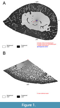 Bone center detection is an important step in the analysis. It can be done manually by using the function BP_ChooseCenter(). However, this method is not recommended as it does not ensure reproducibility of the analysis. Rather, the function BP_DetectCenters() automatically detects the four available centers: section, mineralized, unmineralized, and ontogenetic. The “section” center is the center of the section as defined solely by the outer surface of the bone, the “mineralized” and “unmineralized” centers are the centers of mineralized and unmineralized parts within the section. The center of the section is not generally a correct estimate of the center of the bone that should be used to model compactness, because bone deposition rate on the outer surface and bone resorption rate in the medullary cavity are usually anisotropic. The “ontogenetic” center corrects for this effect and should be the preferred center used for most analyses (Girondot and Laurin 2003). All the detected centers can be shown superimposed on the original image using the function plot() (Figure 1A).
BoneProfileR, like Bone Profiler version 2003, also offers the possibility of processing partial bone sections. This option is particularly useful in certain cases, e.g., when analyzing fossils where only part of the section is preserved, when a bone is complex but relatively homogeneous, or when atypical structures prevent BoneProfileR from correctly measuring bone compactness. Such sections should be drawn like “pie-chart” diagrams. In this case, center position should be specified manually using the BP_ChooseCenter() function and compactness should be estimated using the options center = "user" and partial=TRUE of the function BP_EstimateCompactness().
Compactness Profile
 After the bone center and background and foreground colors have been defined, the compactness profile of the bone section can be estimated. The program uses the bone center (user-specified, section, mineralized, unmineralized, or ontogenetic) as a pivotal point and the compactness is estimated in all directions from that point by shifting the axis along which the pixels are read one pixel at a time, from the edge of the bone to the center, until the whole surface of the section has been covered. Each pixel within the section mask is characterized by its relative distance to the center of the section for that angle and its status (mineralized or not). Pixels are grouped into concentric zones for visualization of observed compactness (Figure 1, Figure 2) but individual pixel information is used to model compactness. BoneProfileR calculates two compactness indices: an observed compactness (the raw number of pixels) and a modeled compactness taking into account the pixel differential representation in the section according to distance to the center.
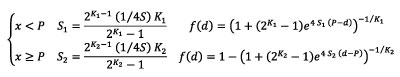
After considering several functions, a scaled logistic function was used in Girondot and Laurin (2003):
![]() (1)
(1)
Where: P is the relative distance from the center to the point where the most abrupt change in compactness is observed. This relative distance is the ratio between the distance to the center and the radius. It generally corresponds to the position of the transition zone between the cortical compacta and the medullary cavity (or spongiosa). S is proportional to the reciprocal of the slope of the compactness change at point P. It usually reflects the width of the transition zone between the cortical compacta and the medullary cavity (or spongiosa). Max is the upper asymptote. It generally reflects the compactness in the outermost cortex. Min is the lower asymptote. It generally reflects the compactness in the center of the medulla.
However, this function constrains the compactness change to be symmetric on both sides of P. A new function named flexit, without this constraint, has been implemented. It has been developed in another context (Abreu-Grobois et al. 2020; Girondot et al. 2021) and has been implemented in BoneProfileR.
The flexit equation is defined as:
 (2)
(2)
The parameters K 1 and K 2 modify the convergence rate of the curve toward asymptotes. When K x <1, the transition toward the asymptote is acute, whereas it is obtuse when Kx >1, with x being 1 (lower asymptote) or 2 (upper asymptote). When the parameters Kx are set to 1, the flexit equation is the same as a logistic equation (1), which ensures backward compatibility of the methods. Equation (2) is a modified form of the original flexit equation (in Abreu-Grobois et al. 2020; Girondot et al. 2021) to ensure that S values from the logistic equation published in Girondot and Laurin (2003) is similar to S from equation (2) when K1 = K2 = 1. If K x is very large, ![]() and
and ![]() are simplified to
are simplified to ![]() and Sx = S Kx /4.
and Sx = S Kx /4.
Then the compactness profile is defined by:
![]() (3)
(3)
The parameters are then P, S, K1, and K2 from equation (2) and Max, Min from equation (3). When equation (1) was used, the width of the spongiosa was directly proportional to the value of S. This is no longer true when equation (3) is used to model compactness because the width of spongiosa also depends on parameters K1 and K2. For this reason, we introduce a new index: the Transitional Range of Compactness l%, or TRC1%, which is the relative width of bone radius (1 is for complete radius) where compacity is between Min + l % X Min and Max - l % X Max. (Equation 4). The value of l% = 0.05 is preferred, but it can be changed by the user:
![]() (4)
(4)
Fitting the Compactness Profile
In Girondot and Laurin (2003), the function was fitted by a Levenberg-Marquart algorithm using the sum of squared differences between observed and modeled compactness values as an adjustment quality measure. We changed the fit criterion to use maximum likelihood and Bayesian analysis to produce better statistics.
During image analysis, it is important to note that each pixel is read only once. A pixel within a section can be mineralized or not; therefore, a binomial distribution is used to estimate the likelihood of a set of pixels using equation 3 as a link function. The maximum likelihood fit is done by successive use of simplex method (Nelder and Mead 1965) and a quasi-Newton method (Fletcher and Reeves 1964). Maximum likelihood (as in BoneProfileR) uses the information at the pixel level whereas sum of squares (as in Bone Profiler) used information at the level of group of pixels. Therefore, models fitted by maximum likelihood are more precise.
As an alternative, the Metropolis-Hastings algorithm is used to estimate the distribution of parameters of equation (3). It is a Markov chain Monte Carlo (MCMC) method for obtaining a sequence of random samples from a probability distribution (Metropolis et al. 1953; Hastings 1970). This method is now widely used as it offers a high-performance tool to fit a model. During the iteration process, a Markov chain is constructed using the estimated parameter values π t, on which a new proposal random function defined by its standard deviation (s) is applied, πt+1 = N (πt, S). This is the Monte-Carlo process. A set of parameters is retained after comparison of likelihood considering priors. It is beyond the scope of this paper to fully explore the fine details of this algorithm; instead, we focus on how to use it.
The choice of the prior is not straightforward (Lemoine 2019) and can be critical if only a few observations are available. However, it is generally not problematic for images because the number of pixels can be very large. A uniform distribution for priors indicates that all values within a range are equally probable, whereas a Gaussian distribution can use a mean and standard deviation obtained from the maximum likelihood analysis of the same section to provide a more informative prior.
The standard deviation (s) for a new proposal is a compromise between two constraints: if the values are too high, the new values could yield results far from the optimal solution, while if they are too low, the model can become stuck in local minima. The adaptive proposal distribution (Rosenthal 2011) as implemented in the R package HelpersMG (Girondot 2021) ensures that the acceptance rate is close to 0.234, which is optimal (Roberts and Rosenthal 2001).
When maximum likelihood is used, the standard error of parameters is obtained by the square-root of the inverse of a Hessian matrix. However, this procedure implies that confidence interval is symmetric, and that error is Gaussian. These hypotheses are no longer necessary when posterior distribution is obtained using a Metropolis-Hastings algorithm. For this reason, estimation of parameters using a Bayesian Metropolis-Hastings algorithm should always be preferred.
Eventually, the user can choose to perform a three-steps analysis, i.e., a quasi-Newton method, a Bayesian MCMC and a second quasi-Newton method, successively. The first step using maximum likelihood estimates a maximum, but it could be a local maximum. The second step using MCMC can eventually escape to a local maximum and the third step computes global maximum likelihood. It generally ensures that global optimum is found but implies a longer computation time.
Statistical Comparison of Profiles
When several models are fitted to the same datasets of observations, the comparison of the performance of the different models can be assayed using AIC (Akaike Information Criterion) (Akaike 1974). AIC is a measure of the quality of fit, while simultaneously penalizing for the number of parameters in the model (Equation 5). It facilitates the selection from a set of models that represent the best compromise between fit quality and over-parametrization.
![]() (5)
(5)
With L j being the likelihood of the model and p j the number of parameters of the model j. When a set of k models are tested, the model with lowest AIC is the best non-overparametrized fit. It is important to note that the AIC value itself is not strictly informative in terms of absolute model fit. When a set of models is compared, it is possible to estimate the relative probability that each model is the best among those tested using the Akaike weight (Burnham and Anderson 2002) (Equation 6):
 (6)
(6)
We use both AIC and Akaike weight to compare the fitted logistic and flexit models.
The utility of model selection can be further extended to test for potential differences in the results from two or more datasets. In this case, the complete data are split into several subsets with each individual dataset being represented once and only once. The test question is: can the collection of datasets be modeled with a single set of parameters, or must each dataset be modeled with its own set? The two alternatives are: (a) are the different datasets similar or (b) not. In this situation, Bayesian Information Criterion (or BIC) should be used instead of AIC, because the true model is obviously among the tested alternatives (Equation 7).
BIC = -2 ln L + p ln n (7)
When the BIC statistic is used, all the priors of the models tested are assumed to be identical. It is also possible to estimate BIC weights by replacing AIC with BIC in the Akaike weight formula. The w -value has been defined as the probability that several datasets can be correctly modeled by grouping the datasets instead of modeling them independently of each other; it is calculated using BIC weights (Girondot and Guillon 2018).
Radial Compactness Profile
When analyzing some bone sections, we have noticed that the pattern of bone compactness was not uniform for all angles. In this situation, the fitted global model represents an average of the compactness change, and the interpretation of the S parameter is complex because it includes three components: the slope of the transition from cortex to medulla, the angular variability of the S parameter, and the angular variability of the P parameter.
To circumvent these problems, we developed a radial analysis of bone compactness profile. Basically, it is the same as analyzing bone compactness, but the model is applied successively to x slices of bone section representing an angle of 2π/x radians (Figure 1). Then a radial series of parameter values are reported. The user has the possibility to define the reference for the radial analysis. By default, the right and left of the section are respectively located at 0 and pi, and the bottom and top at pi/2 and -pi/2. The R version also allows the user to graphically visualize the model fit for a given angle.
Storing Results
BoneProfileR uses the new results management system (RM) introduced in HelpersMG R package version 4.1: all the results are stored as part of the analyzed image. This result management software has been developed to help users store the results associated with the method used to obtain them (type of center used, background and foreground colors). It is part of the large movement in science of replicative research (Amaral and Neves 2021). An analysis is stored with the image in a single file with all the necessary information to reproduce the analysis. Several analyses can be stored within a single object. They can be called using the parameter “analysis” available for most of the functions of BoneProfileR. The results of an analysis can be exported as a pdf file or as an XML spreadsheet compatible with Open Office or Microsoft Office.
RESULTS
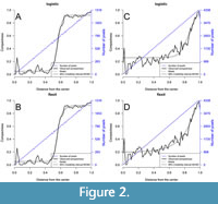
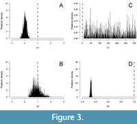 The new compactness model has been applied to the femur of an extant hedgehog (Erinaceus europaeus) and a Permian temnospondyl (Eryops megacephalus). Figure 1 shows (A) the automatic detection of centers in a femur section of the hedgehog (Erinaceus europaeus) and (B) the user-specified center in the femur section of Eryops megacephalus. Then, logistic and flexit models were fitted for these bone sections using the ontogenetic center (Figure 2). The models seem similar when compared visually for Erinaceus europaeus (Figure 2A, B) but the AIC and Akaike weight indicate that flexit model is selected (p=1; Table 1A). The flexit model is also selected for Eryops megacephalus (p=1; Table 1B), and the difference between logistic and flexit modelscan be easily visualized (Figure 2C, D). The posterior distributions of K1 and K2 parameters of the Bayesian Metropolis-Hastings method applied to the Erinaceus europaeus femur show that K1 is indeed always lower than 1 (Figure 3A), which is the value to convert a flexit model into a logistic one. This result confirms that the flexit model best fits the data, as shown in Table 1A. For Eryops megacephalus, the posterior distribution of K2 parameters is well-defined (Figure 3D) but the posterior distribution of K1 is much wider (Figure 3C). The origin of the large range of Kx posterior values lie in equation 3: the output of equation 3 is nearly insensitive to exact Kx value (taking into account the digit precision of computer) as long as Kx is large. However, the information conveyed by Kx is only pertinent when combined with Sx to produce the new TRCl% index; Kx should not be used in paleobiological modeling. In this case, the difficulties on the use of Kx disappear.
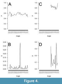 The posterior distributions of P and S are mean=0.559, SD=0.0001 and mean=0.028, SD=0.001, respectively, for flexit model applied to Erinaceus europaeus and mean=0.849, SD=0.001 and mean=0.082, SD=0.001 for the flexit model applied to Eryops megacephalus. However, as explained previously, the S value informs both on the real transition from cortex to medulla but also on the radial diversity of P and S values. The fitted P and S values of radial analysis of bone compactness show the angular variability in these parameters (Figure 4). As expected, the posterior distribution of P from the global analysis is similar to the distribution of P from radial analysis for both Erinaceus europaeus (mean=0.556, SD=0.045) and Eryops megacephalus (mean=0.836, SD=0.053) (Figure 4A, C). On the contrary, the fitted values of S for radial analysis shows great variability, with outliers (Figure 4B, D). They range from 0.0002 to 0.30, with a median of 0.009 for Erinaceus europaeus (Figure 4B). This last value is much lower than the fitted value for the global analysis (mean=0.028, SD=0.001). The same pattern is observed for Eryops megacephalus (radial analysis: range for S values between 0.0001 and 0.90, median=0.089; global analysis: mean=0.082, SD=0.001) (Figure 4D). The median S value from a radial analysis, the average global S value, and the transitional range of compacity could be used for further analyses, as they do not convey the same information.
Erinaceus europaeus has a P and S reflecting a relatively thick cortex and an abrupt medullo-cortical transition. Biologically, this corresponds to a weak development of a spongiosa in the periphery of the medullary region (Figure 1A), which is generally characteristic of terrestrial organisms. Eryops megacephalus has a thinner cortex and a more gradual transition zone between medulla and cortex (higher P and S than in Erinaceus). In fact, the femur section of Eryops shows a prominent spongiosa (Figure 1B) characteristic of some aquatic organisms. Moreover, the lifestyle of Eryops was inferred to be aquatic by all models presented in the study by Quemeneur et al. (2013) based on the compactness parameters calculated by the first version of Bone Profiler. These conclusions (at least regarding the values of parameters P and S) are confirmed by the present study.
DISCUSSION
As for many biological objects, bone cross-sections are complex, and their quantitative description requires going beyond a subjective expert opinion. The method and software proposed here has many advantages. First, it can standardize the method used to analyze bone sections. For example, no objective method has been described to determine where the cortical compacta ends and where the cancellous bone begins. Thus, cortical thickness and compactness measurements given by various authors are difficult to compare, unless there is no cancellous bone. Second, the program can model the bone compactness profile to test biological hypotheses. However, it is always important to keep in mind that models are simplifications or approximations of reality and hence will not reflect all of reality (Burnham and Anderson 2002). Box (1979) noted that “all models are wrong, but some are useful.” The large range of publications using the Bone Profiler model shows that this model is useful.
In conclusion, the new methods implemented in BoneProfileR enhance the bone compactness model published in Girondot and Laurin (2003). This update introduces new statistically sound methods (maximum likelihood, Bayesian analysis), a new function to model compactness, and a new radial analysis to estimate the parameters of bone compactness. The new software is an R package, and data can be directly used in statistical analyses considering phylogeny for example. A user-friendly Web-version is also available, but it gives access to only a subset of the options available through the command line interface (CLI) version within R.
ACKNOWLEDGMENTS
The authors would like to thank the referees (E. Amson, D. Hoffman, and the third anonymous referee) for their valuable comments which helped to improve the manuscript. We thank also the handling editor, Heinrich Mallison, for his help to publish this manuscript.
REFERENCES
Abreu-Grobois, F.A., Morales-Mérida, B.A., Hart, C.E., Guillon, J.-M., Godfrey, M.H., Navarro, E., and Girondot, M. 2020. Recent advances on the estimation of the thermal reaction norm for sex ratios. PeerJ, 8:e8451. https://doi.org/10.7717/peerj.8451
Akaike, H. 1974. A new look at the statistical model identification. IEEE Transactions on Automatic Control, 19:716-723. https://doi.org/10.1109/tac.1974.1100705
Amaral, O.B. and Neves, K. 2021. Reproducibility: expect less of the scientific paper. Nature, 597:329-331. https://doi.org/10.1038/d41586-021-02486-7
Amson, E., de Muizon, C., Laurin, M., Argot, C., and de Buffrénil, V. 2014. Gradual adaptation of bone structure to aquatic lifestyle in extinct sloths from Peru. Proceedings of the Royal Society B-Biological Sciences, 281(1782):20140192. https://doi.org/10.1098/rspb.2014.0192
Box, G.E.P. 1979. Robustness in the strategy of scientific model building, p. 201-236. In Launer, R.L. and Wilkinson, G.N. (eds.), Robustness in Statistics. Academic Press, New York.
Burnham, K.P. and Anderson, D.R. 2002. Model selection and multimodel inference: A practical information-theoretic approach. Springer-Verlag, New York.
Castanet, J. and Caetano, M.H. 1995. Influence du mode de vie sur les caractéristiques pondérales et structurales du squelette chez les amphibiens anoures. Canadian Journal of Zoology, 73:234-242. https://doi.org/10.1139/z95-027
Chinsamy, A. and Warburton, N.M. 2021. Ontogenetic growth and the development of a unique fibrocartilage entheses in Macropus fuliginosus. Zoology, 144:125860. https://doi.org/10.1016/j.zool.2020.125860
de Buffrénil, V. and Francillon-Vieillot, H. 2001. Ontogenetic changes in bone compactness in male and female Nile monitors (Varanus niloticus). Journal of Zoology, 254:539-546. https://doi.org/10.1017/s0952836901001042
de Ricqlès, A.J. 2021. Paleohistology: An historical-bibliographical introduction. In de Buffrénil, V., Zylberberg, L., de Ricqlès, A.J., Padian, K., Laurin, M., and Quilhac, A. (eds.), Vertebrate Skeletal Histology and Paleohistology. CRC Press, Boca Raton.
Faure-Brac, M.G. and Cubo, J. 2020. Were the synapsids primitively endotherms? A palaeohistological approach using phylogenetic eigenvector maps. Philosophical Transactions of the Royal Society B-Biological Sciences, 375(1793):20190138.
https://doi.org/10.1098/rstb.2019.0138
Fletcher, R. and Reeves, C.M. 1964. Function minimization by conjugate gradients. Computer Journal, 7:148-154. https://doi.org/10.1093/comjnl/7.2.149
Girondot, M. 2021. HelpersMG: Tools for Environmental Analyses, Ecotoxicology and Various R Functions. The Comprehensive R Archive Network.
Girondot, M. and Guillon, J.-M. 2018. The w-value: An alternative to t- and χ2 tests. Journal of Biostatistics & Biometrics, 1(1):1-4.
Girondot, M. and Laurin, M. 2003. Bone profiler: a tool to quantify, model, and statistically compare bone-section compactness profiles. Journal of Vertebrate Paleontology, 23:458-461. https://doi.org/10.1671/0272-4634(2003)023[0458:bpattq]2.0.co;2
Girondot, M., Mourrain, B., Chevallier, D., and Godfrey, M.H. 2021. Maturity of a Giant: Age and size reaction norm for sexual maturity for Atlantic leatherback turtles. Marine Ecology, 42(5):e12631. https://doi.org/10.1111/maec.12631
Hastings, W.K. 1970. Monte Carlo sampling methods using Markov chains and their applications. Biometrika, 57(1):97-109. https://doi.org/10.1093/biomet/57.1.97
Houssaye, A., Waskow, K., Hayashi, S., Cornette, R., Lee, A.H., and Hutchinson, J.R. 2016. Biomechanical evolution of solid bones in large animals: a microanatomical investigation. Biological Journal of the Linnean Society, 117(2):350-371. https://doi.org/10.1111/bij.12660
Jaquier, V.P. and Scheyer, T.M. 2017. Bone histology of the Middle Triassic long-necked reptiles Tanystropheus and Macrocnemus (Archosauromorpha, Protorosauria). Journal of Vertebrate Paleontology, 37(2):e1296456. https://doi.org/10.1080/02724634.2017.1296456
Laurin, M., Girondot, M., and Loth, M.-M. 2004. The evolution of long bone microstructure and lifestyle in lissamphibians. Paleobiology, 30(4):589-613.
Lemoine, N.P. 2019. Moving beyond noninformative priors: why and how to choose weakly informative priors in Bayesian analyses. Oikos, 128(7):912-928. https://doi.org/10.1111/oik.05985
Metropolis, N., Rosenbluth, A.W., Rosenbluth, M.N., Teller, A.H., and Teller, E. 1953. Equation of state calculations by fast computing machines. Journal of Chemical Physics, 21(6):1087-1092. https://doi.org/10.1063/1.1699114
Nelder, J.A. and Mead, R. 1965. A simplex method for function minimization. The Computer Journal, 7:308-313. https://doi.org/10.1093/comjnl/7.4.308
Nolan, R. and Padilla-Parra, S. 2018. ijtiff: An R package providing {TIFF} I/O for {ImageJ} users. Journal of Open Source Software, 3(23):633. https://doi.org/10.21105/joss.00633
Quémeneur, S., Buffrénil, V. de and Laurin, M.. 2013. Microanatomy of the amniote femur and inference of lifestyle in limbed vertebrates. Biological Journal of the Linnean Society 109:644–655. https://doi.org/10.1111/bij.12066
Roberts, G.O. and Rosenthal, J.S. 2001. Optimal scaling for various Metropolis-Hastings algorithms. Statistical Science, 16(4):351-367. https://doi.org/10.1214/ss/1015346320
Rosenthal, J.S. 2011. Optimal proposal distributions and adaptive MCMC, p. 93-112. In Brooks, S., Gelman, A., Jones, G., and Meng, X.-L. (eds.), MCMC Handbook. Chapman and Hall/CRC
Rueden, C.T., Schindelin, J., Hiner, M.C., DeZonia, B.E., Walter, A.E., Arena, E.T., and Eliceiri, K.W. 2017. ImageJ2: ImageJ for the next generation of scientific image data. BMC Bioinformatics, 18(1):529. https://doi.org/10.1186/s12859-017-1934-z
