Residual diversity simulation

A simulation-based examination of residual diversity estimates as a method of correcting for sampling bias

Neil Brocklehurst

Article number: 18.3.7T
https://doi.org/10.26879/584
Copyright Palaeontological Association, November 2015

Author biography
Plain-language and multi-lingual abstracts
PDF version

Submission: 3 July 2015. Acceptance: 30 October 2015

{flike id=1357}

ABSTRACT

The influence of sampling biases on estimates of species richness through geological time is a great concern, and multiple methods have been developed to correct for them. One method is the residual diversity estimate, a modelling approach which removes the signal of a chosen sampling proxy. Despite having been widely applied to palaeodiversity studies, the residual diversity estimate has yet to be tested in a simulation environment. One difficulty with such a test is that the simulation must model sampling in such a way that a sampling proxy may be extracted from the model in order to calculate the residual diversity. Here, a novel approach is used to examine the efficacy of this method. Taxa and an associated phylogeny were simulated using a birth-death model, and a parameter was added representing dispersal of the taxa between areas in simulated space. The simulated space in each time bin was divided into formations and localities, which were removed at random to represent incomplete sampling, also providing sampling proxies used to calculate the residual diversity estimate. The residual diversity estimate is found to perform best when the broader proxy representing entire regions, e.g., formations, is used in its calculation, rather than more restricted localities. A recent update to the residual diversity estimate, incorporating polynomial relationships between diversity and proxies, performs poorly, sometimes showing a worse correlation with the true diversity than the raw data. The residual diversity estimate is consistently outperformed by the phylogenetic diversity estimate, even when errors are introduced to the phylogeny.

Neil Brocklehurst. Museum für Naturkunde, Leibniz-Institut für Evolutions- und Biodiversitätsforschung, Invalidenstraße 43, 10115 Berlin, Germany, neil.brocklehurst@mfn-berlin.de

Keywords: species richness; diversity; simulation; residual diversity estimate; phylogenetic diversity estimate; sampling correction

Final citation: Brocklehurst, Neil. 2015. A simulation-based examination of residual diversity estimates as a method of correcting for sampling bias. Palaeontologia Electronica 18.3.7T: 1-15. https://doi.org/10.26879/584
palaeo-electronica.org/content/2015/1357-residual-diversity-simulation

INTRODUCTION

Understanding changes in species richness through geological time is of paramount importance when studying the evolutionary history of a clade. Such investigations enable palaeontologists to deduce the major events in the history of the group under study and are also relevant to broader questions, such as the impact of and recovery from mass extinctions, the processes underlying evolutionary radiations and the importance of competition and co-evolution. Such questions, however, are hampered by the incompleteness of the fossil record. This incompleteness has long been acknowledged, but it was not until the seminal paper of Raup (1972) that consideration was given towards how the incompleteness of the fossil record may be impacting on our interpretations of it in a systematic and, more importantly, correctable manner. Raup (1972) suggested two methods to deal with this issue: modelling and subsampling.

Subsampling has been widely used both in palaeontology and neontology, and the performance of various implementations has been extensively examined, both using simulations and case studies (Sanders, 1968; Smith et al., 1985; Miller and Foote, 1996; Alroy et al., 2001, 2008; Chao et al., 2009; Zhang and Stern, 2009; Alroy, 2010a, 2010b). The most widely used in palaeontology has been rarefaction (Sanders, 1968), although recently Alroy (2010a, 2010b) proposed the Shareholder Quorum method, which was shown to perform better than rarefaction under hypothetical situations and simulation studies, as well as being applied to real data.

The use of modelling in sampling correction was not explored in great detail until Smith and McGowan (2007) introduced the residual diversity estimate. This approach requires a proxy for sampling bias such as number of collections or formations or outcrop area in each time bin. A model diversity estimate, based on a perfect linear relationship between diversity and the chosen sampling proxy, is produced by sorting both diversity and proxy data from low to high and fitting a linear model. The model diversity estimate is then subtracted from the observed diversity, leaving the residual diversity estimate. The idea behind this method is that the observed diversity estimate is a signal of both sampling and the actual diversity. Subtracting the model diversity estimate in theory removes the sampling signal, leaving only the biological signal (Smith and McGowan, 2007).

The residual diversity method has proven popular, particularly in analyses of terrestrial vertebrate datasets where sample sizes are sometimes too small for subsampling (Smith and McGowan, 2008; Barrett et al., 2009; Butler et al., 2009, 2011; Wall et al., 2009; Benson et al., 2010; Brocklehurst et al., 2012, 2013; Benson and Upchurch, 2013; Fröbisch, 2013, 2014; Pearson et al., 2013). Lloyd (2012) refined the method, allowing for non-linear relationships between the sampling proxy and diversity, and also introducing confidence intervals to show which peaks and troughs are significant. However, despite its popularity, there has never been a thorough test demonstrating that this method does produce an accurate estimate of palaeodiversity in the same way that the performance of subsampling methods has been tested in simulation studies. A third sampling correction method, the phylogenetic diversity estimate, in which ghost lineages are incorporated into the diversity estimate, thus including as yet unsampled portions of the fossil record which may be deduced from a phylogeny, has been tested in a simulation environment (Lane et al., 2005). The residual diversity estimate and Lloyd’s alteration thereof, however, have only been examined in the context of applying these methods to real data, or comparing the diversity curves produced to other methods (Smith et al., 2012). This is obviously an unsatisfactory test; we do not know the true palaeodiversity, so we have no way of knowing if the residual diversity estimate is in fact producing a true signal. Such confirmation can only be provided by simulated data subjected to simulated sampling bias, where the similarity between the sampling corrected and the known true diversity signals can be measured.

This study represents the first rigorous test of the performance of the residual diversity estimate under a variety of sampling conditions. Its performance is compared to a raw estimate of diversity (no sampling correction) and also to the phylogenetic diversity estimate. Both the original method proposed by Smith and McGowan (2007) and the refinement by Lloyd (2012) are subjected to the same tests.

MATERIALS AND METHODS

Simulation-based studies of subsampling methods and the phylogenetic diversity estimate have simply required data points to be deleted at random. A simulation-based analysis of the residual diversity estimate is made complicated by its implementation; the method uses a proxy for sampling to create the model diversity estimate, which is subtracted from the observed diversity estimate. Such proxies include attempts to quantify human sampling effort such as the number of fossil-bearing collections in each time bin (Crampton et al., 2003; Butler et al., 2011; Brocklehurst et al., 2012, 2013) or geological biases such as rock outcrop area (Peters and Foote, 2001; Smith, 2001; Crampton et al., 2003; Smith and McGowan, 2007, 2008; Wall et al., 2009; Fröbisch, 2013, 2014) or number of formations dated to each time bin (Fröbisch, 2008; Barrett et al., 2009; Butler et al., 2009; Benson et al., 2010; Mannion et al., 2011; Benton, 2012; Benson and Upchurch, 2013). Therefore, to examine the residual diversity estimate in a simulation environment, one cannot simply delete taxa at random in each time bin. One must simulate sampling in such a way that a sampling proxy may be extracted from the model, a proxy which approximates the biases affecting the real-world fossil record. Here, a novel simulation environment is proposed in order to simulate such proxies.

The simulation is based on an expansion of the simFossilTaxa function in the R package paleotree (Bapst, 2012). This function implements a stochastic birth-death model; at any one point in time, a taxon may undergo speciation, either by budding (a new species branches off from the original, while the original remains), cladogenesis (a species diverges into two lineages which both represent different taxa to their parent) or anagenesis (one species gives rise to a single descendant species). Also, at any point in time, any taxon may go extinct. In the simulation presented herein, the probability of speciation and extinction are set equal, and each mode of speciation has an equal probability. Thus, variation in diversity occurs by a random walk. No size limit was placed on the clade generated in this model, but only clades surviving for 50 units of simulated time were retained for the analyses.

An additional two parameters are added to the model presented in the original R package: random dispersal and local extinction. An area of simulated space is generated, divided into 10 regions. When a new species is produced in the simulation, it is randomly assigned to a region of origin. At any point in time, this species may disperse (expand its range to another area) or it may undergo regional extinction (die out in only one region whilst remaining in any other regions it happens to occupy). The probability of dispersal relative to the probability of local extinction is hereafter referred to as PD/PLE (see Table 1 for the full list of abbreviations used in the text and figures) and is a variable parameter in the simulations (see Table 2 for the full list of parameter variations in each simulation).

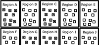
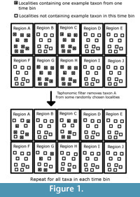This model outputs a clade that has evolved over time and space. The period of simulated time is then divided into 50 time bins, and the number of lineages present in each time bin is counted. This provides the “true diversity,” the signal which palaeontologists hope to emulate. Then a novel method of simulating sampling is applied. Each region in sampling space and each time bin is taken to represent a rock formation of a specific age that can produce fossils. Each of these “formations” is split into 10 “localities”. Each species present in that time bin starts as present in every locality of the regions it occupied. Then, the simulated space in each time bin passes through three simulated sampling filters, each representing a different bias affecting the fossil record. The first of these filters represents the taphonomic processes which lead to the elimination of individuals before the fossilisation process. Each species may be randomly deleted from any locality it inhabited with the probability “PTAPH” (probability variable in simulations). An example of how the taphonomic filter may be applied to one species in one time bin is shown in Figure 1. The second filter represents geological biases; fossil-bearing formations may be destroyed by erosion or subduction before sampling occurs, or covered by further sedimentation. Each of the simulated formations (and the “fossils” within) is therefore subjected to random deletion with a probability “PFORM” (variable parameter). The final filter represents human sampling biases; not all fossil-bearing localities have been explored. Therefore, each locality (and the “fossils” within) is subjected to random deletion with a probability “PLOC” (variable parameter). An example of how these final two filters may be applied to one time bin is shown in Figure 2.

This method of simulating sampling allows two sampling proxies to be output, along with diversity data. One may count those formations and localities in each time bin, which were not randomly deleted and are, therefore, contributing to the diversity count.

Those taxa remaining in each time bin after three rounds of random deletion make up the palaeontological dataset: the fossils representing what palaeontologists have found in a biased fossil record. From this data, 10 different diversity curves are produced. Each of these 10 curves is compared to the “true” diversity (diversity before the sampling filters are applied) using the Spearman’s rank correlation coefficient. The Spearman’s rho value is used as a measure of how closely each diversity curve represents the true palaeodiversity. The 10 diversity curves are described below.

The Taxic Diversity Estimate

No sampling correction method is applied. This represents raw count of the number of species sampled in each time bin; that is, the observed fossil record including all the biases.

The Phylogenetic Diversity Estimate

This method corrects for sampling by incorporating ghost lineages into the diversity estimate. Ghost lineages are lineages which are not observed in the fossil record, but are inferred to be present from a phylogeny based on the assumption that two taxa must have split from their common ancestor at the same time (Norrell, 1992). Therefore, if one taxon is observed in the fossil record at a particular time, its sister taxon may be inferred to have been present at that time bin as well, even if it is not observed in the fossil record until later. Including these ghost lineages in a diversity estimate includes as yet unsampled portions of the fossil record (Smith, 1994). Use of this method is obviously limited to clades for which a comprehensive phylogeny exists, and as such it has been most widely applied to vertebrates (Upchurch and Barrett, 2005; Lloyd et al., 2008; Barrett et al., 2009; Benson et al., 2010; Mannion et al., 2011; Ruta et al., 2011; Brocklehurst et al., 2013; Walther and Fröbisch, 2013). The phylogenetic diversity estimate has been shown to be more accurate than the taxic diversity estimate in simulation studies (Lane et al., 2005) and, therefore, provides a benchmark for comparison with the residual diversity estimate. The two are used on similar datasets and multiple studies have applied both to the same dataset (Barrett et al., 2009; Mannion et al., 2011; Brocklehurst et al., 2013).

The taxa2cladogram function in paleotree was used to produce a cladogram from the output of the birth-death model. The cladogram produced by this function takes into account how ancestor descendant relationships are resolved using current phylogenetic methods; ancestors are resolved as the sister to, or in a polytomy with, the descendants depending on what mode of speciation separated them (Bapst, 2013). The tree is time calibrated using the reduced ranges of taxa resulting from the sampling filters (those taxa not sampled at all are pruned from the tree). Ghost lineages are inferred and phylogenetic diversity estimate is calculated.

The Lane et al. (2005) test of the phylogenetic diversity estimate assumed a correct phylogeny. In this analysis, error is incorporated into the phylogeny using random nearest neighbour interchange applied to each node with a probability of PMIST (variable parameter). This was implemented using the function rNNI in the R package phangorn (Schliep, 2011).

The Residual Diversity Estimate

Eight different implementations of the residual diversity estimate are tested, taking into account three variables: the method used to calculate residuals, the sampling proxy used and the inclusivity of the sampling proxy.

Method. Two implementations of the residual diversity estimate have been suggested. The first, that of Smith and McGowan (2007), hereafter called the Smith and McGowan method, calculates a model diversity estimate assuming a linear relationship between sampling and observed diversity. It is also assumed that deviations from this observed linear relationship represent genuine diversity changes in history. Lloyd (2012) suggested that one should not assume a linear relationship. Instead, non-linear models are tested and the best fitting model is calculated using the Akaike Information Criterion (hereafter this method is referred to as the Lloyd method).

Sampling proxy. The model outputs two sampling proxies. The first represents the number of formations through time and the second the number of localities through time. While the model obviously cannot perfectly represent the vagaries of human sampling, testing the output of both proxies by the simulation provides a comparison between the broader (formations) and the narrower (localities) proxy.

Inclusivity of the proxies. A potential problem has been raised concerning the use of the residual diversity estimate: redundancy (Benton et al., 2011; Benton, 2012; 2015; Dunhill et al., 2014). It has been argued that the sampling proxies used are not independent of the data they seek to correct. If, for example, dinosaur diversity did actually decrease, one would expect there to be fewer dinosaur-bearing formations (Benton et al., 2011). Moreover, in using dinosaur-bearing formations as a proxy to correct for biases in dinosaur diversity, the researcher does not take into account occasions when workers have looked at rocks of a particular age but have not found dinosaurs. To resolve this problem, some workers have suggested more inclusive proxies should be used (Upchurch and Barrett, 2005; Brocklehurst et al., 2012, 2013). For example, Brocklehurst et al. (2013) used amniote-bearing collections as a proxy when calculating the residual diversity estimate of synapsids, thus including occasions where workers had examined rocks containing fossils of taxa closely related to synapsids, but not found any synapsids. The effectiveness of this method is examined here; residual diversity estimates are first calculated from proxies including only those formations and localities in which fossils of the simulated clade remain, and secondly using all formations and localities which were not subjected to random deletion, even if the taphonomic filter had removed all the fossils in some of these (see Figure 2 for the distinction between these proxies).

When all possible combinations of these three parameters are applied, there are eight possible versions of the residual diversity estimate. All tested in this study.

Parameter Variations

A list of the parameter variations tested in this study is presented in Table 1. For each set of parameters, 100 simulations were carried out. Each simulation produced all 10 diversity curves. Each of these 10 curves was compared to the true diversity using the Spearman’s rank correlation coefficient. Therefore, for each of the 10 methods of inferring diversity, 100 rho values were produced for each set of parameters. The mean of these rho values provided a measure of the performance of each of these methods under the parameters tested. The mean and standard deviation Spearman’s rho values for each diversity estimate in each set of parameters, is presented in Appendix.

RESULTS AND DISCUSSION

Methods of Implementing the Residual Diversity Estimate

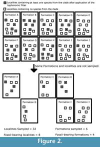
The relative performance of the eight different methods of carrying out the residual diversity estimate showed a number of consistent patterns. One clear result is a rejection of the Lloyd method of calculating residuals, incorporating polynomial relationships between observed diversity and the sampling proxy. In most sampling regimes tested, and no matter what sampling proxy is used, the Lloyd method performs worse than the Smith and McGowan method (Figure 3.1-2). In fact, when sampling is low, some simulations resulted in a negative relationship between the true diversity and the residual diversity estimates calculated using the Lloyd method. At most levels of sampling, the Smith and McGowan method provides a much closer correlation with the true diversity, with mean Spearman’s rho values sometimes almost double those obtained when the Lloyd method is used. At low levels of sampling, however, the difference in performance is greatly reduced, and the rho values obtained using each method are more similar, or in some cases the Lloyd method produces a slightly higher mean rho value.

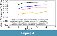The Smith and McGowan method assumes a linear relationship between sampling and observed diversity, whereas the Lloyd method makes no such assumption. Instead the Lloyd method tests for both linear and polynomial relationships. One might argue that the simple model of sampling presented here does not represent true sampling heterogeneity, and that the Lloyd method might perform better in the “real world”. The sampling of localities and formations in the simulation is random, whilst in reality there are areas, formations and continents which receive considerably more attention than others (Benton et al., 2011; Brocklehurst et al., 2012; Dunhill et al., 2013). On the other hand, if the Lloyd method cannot perform under this simplest of sampling regimes, one cannot really trust its performance in more complicated situations. If the simulated sampling regime was causing a linear relationship between the proxy and observed diversity, the Lloyd method should have detected this and produced the same result as the Smith and McGowan method. Instead, we must infer that the simulation is producing proxies and taxic diversity estimates with a polynomial relationship, but the polynomial relationship does not relate to sampling; if it did, the Lloyd method should outperform the Smith and McGowan method. Lloyd (2012) did note that the modelled relationship might incorporate some genuine biological signal as well as sampling signal. It is also possible that the polynomial relationships are a result of the varying signals of provinciality and distribution in each time bin; in other words they represent a genuine biological signal. Therefore, correcting for a polynomial relationship is removing an aspect of the true signal, leading to a worse performance. This may explain the improved performance of the Lloyd method relative to the Smith and McGowan method at lower sampling levels; when sampling is very poor one is less likely to find multiple specimens of the same species from multiple regions (although it should be noted that both show reduced rho values at low sampling levels). Supporting this inference is the fact that, as the rate of dispersal relative to the rate of local extinction increases (that is, the faunas become more homogenous), the gap in performance between the Smith and McGowan method and the Lloyd method increases (Figure 4).

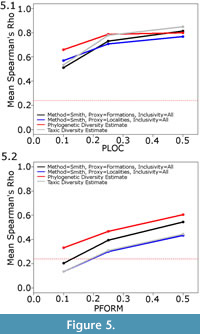The second issue to consider is the choice of proxy. At almost all sampling levels and using both the Smith and McGowan and Lloyd methods, the simulated formations are found to be a better proxy than the simulated localities (Figure 3). The only sampling regime where localities were found to perform better as a proxy than formations is when locality sampling was forced to be the dominant influence on sampling (PFORM and PTAPH were set to 0.9, and PLOC was set considerably lower; Figure 5.1). Even under these conditions, it was only at low sampling levels that localities were found to outperform formations as a proxy.

One must be careful about interpreting this result; this cannot be taken as a simple endorsement of formations as a proxy over localities. This simulation, while including considerably more parameters than previous examinations of sampling correction methods, can obviously not recreate perfectly the vagaries of human sampling, or the inconsistencies surrounding the human definitions of “formations”, “basins” and “members”. Formation counts have been criticised as being extremely arbitrarily defined, with formations varying by up to eight orders of magnitude in volume (Peters, 2006; Peters and Heim, 2010; Benton et al., 2011; Dunhill, 2012). Crampton et al. (2003) demonstrated that the number of formations poorly represents sedimentary outcrop area. In fact, rock outcrop area measured from geological maps only approaches the area of rock that is exposed and available for study under certain conditions e.g., low soil coverage (Dunhill, 2012). Benton et al. (2013) provided a detailed comparison of a variety of proxies for the quality of the rock record, including formation counts from various sources, rock outcrop area and counts of rock units from the Macrostrat database, where units representing hiatus bound sedimentary rock packages (Peters and Heim, 2010). These different proxies, supposedly assessing similar biases, showed great variation in the strength of their correlation to each other and to tetrapod diversity.

Nevertheless, the fact that the simulated formations consistently outperform simulated localities when used to calculate the residual diversity estimate may still be an important result when considering proxy choice. The key issue is that the “formations” are the broader proxy, representing entire areas of simulated space with distinct faunas. While the simulation allows movement of species between these areas, range size is limited by the potential for local extinction, which occurs with an equal probability to dispersal in the simulations shown in Figure 3. Thus, simulated species tend to have restricted ranges, a result which mirrors the real world (Preston, 1962; Raup, 1972). Therefore, when an entire formation is removed in the simulation, or not sampled in the real world, one is potentially removing an entire set of species endemic to that region. On the other hand, if a locality within a formation is not sampled, this does not preclude the possibility of sampling the endemic species; there is still potential at other localities. It is interesting to note that, when the rate of dispersal is increased relative to the rate of local extinction, the gap between the performance of formations and localities as a proxy decreases, albeit only slightly (Figure 4). Dunhill et al. (2014) have already argued that formations are less redundant with the true diversity than the localities and collections. While one must remember the simulated nature of the results here, both the simulation and consideration of real data would imply the need to consider sampling proxies which cover broader areas rather than single quarries or localities. This does not, however, mitigate the concerns surrounding the arbitrary nature of formation definitions.

The final consistent pattern discussed here is the breadth of the sampling proxy. As discussed above, a number of workers have attempted to correct for the issue of redundancy by using broader sampling proxies e.g., using dinosaur-bearing collections as a proxy when calculating a residual diversity estimate of Mesozoic birds (Brocklehurst et al., 2012). The idea behind such a method is that, if one only includes formations or localities in which fossils of the clade of interest have been found, one is not representing the full extent of the sampling that has been undertaken. Many areas will have been examined that have produced no fossils of the clade in question, but still represent sampling effort. Broadening sampling proxies to areas that have produced fossils of a broader clade, one containing the clade of interest, allows the inclusion of formations which both have preserved and also have the potential to preserve fossils of the chosen clade, a more accurate representation of sampling.

The use of such broader proxies is supported here. Under all sampling regimes, both the Lloyd and Smith and McGowan methods and using either formations or localities as a proxy, a better correlation with the true diversity is obtained when the sampling proxy includes all localities/formations which were not subjected to random deletion (Figure 3), whether or not a simulated fossil was “found” in it. The difference is substantial; in fact, including only those formations/localities which have produced fossils consistently gives a lower mean score than the taxic diversity estimate, indicating that using the more restricted sampling proxy produces a residual diversity estimate further from the true diversity than an uncorrected diversity curve. It appears that merely counting the number of formations and localities which preserve fossils of your clade of interest is not only a poor representation of sampling, but it is producing highly spurious results which are a worse representation of history than the raw data.

Comparing the Residual Diversity Estimate to Other Methods

The results described above provide information on how one might best implement the residual diversity estimate. Under the majority of sampling regimes, the highest mean Spearman’s rho of the eight residual diversity implementations was found when formations were used as a sampling proxy, when the Smith and McGowan method was used, and when all formations not subjected to random removal were incorporated rather than just those containing a fossil. But how does this implementation of the residual diversity estimate compare to other diversity estimates?

This optimum implementation of the residual diversity estimate consistently outperforms the raw, taxic diversity estimate (Figure 3), although the correlation of both with the true diversity estimate decreases as the sampling probabilities decrease, and the decrease occurs at a similar rate. This method is indeed an appropriate method to correct for sampling and can provide a better representation of the true history of a clade than the raw data. It should be noted that the performance of the taxic diversity estimate does not lag far behind this optimum implementation of the residual diversity estimate and outperforms many of the other possible implementations (Figure 3).

The phylogenetic diversity estimate, however, consistently outperforms both of the other methods (Figure 3.4). Under most sampling regimes, the phylogenetic diversity estimate shows a better correlation with the true data than either the residual or the taxic diversity estimate. This is despite the fact that the phylogeny used in its estimation is not the true representation of the relationships; instead, ancestors are found to be the sister to or in a polytomy with their descendants, as would occur in phylogenetic analyses using current methods (Bapst, 2013). Even when formations are forced to be the dominant influence on sampling (PLOC and PTAPH are set to 0.9, while PFORM is set considerably lower), the residual diversity estimate using formations does not correlate better with the true data than the phylogenetic diversity estimate (Figure 5.2). Moreover, although the correlation of the phylogenetic diversity estimate with the true data does decrease with worse sampling, the rate of decrease is less than that of the taxic or residual diversity estimates. It appears the phylogenetic diversity estimate is more robust to poor sampling than either of these alternative methods.

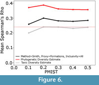Additionally, the phylogenetic diversity estimate appears to be remarkably resistant to errors in the phylogeny (Figure 6). Although its correlation with the true data did decrease as more errors were incorporated, the decrease is not at all substantial. Even with the error rate rising to 50%, the phylogenetic diversity estimate still showed a better correlation with the true data than either the taxic or residual diversity estimate.

While this simulation does appear to be clearly endorsing the phylogenetic diversity estimate over the residual diversity estimate, there are other issues which need to be acknowledged. Although the phylogenetic diversity estimate does correlate better with the true diversity estimate and, therefore, provides a better representation overall, there are issues with the phylogenetic diversity estimate which cannot be detected with a simple correlation test. First it has been shown that the phylogenetic diversity estimate is more heavily influenced than other estimates by the Signor Lipps effect, where rapid extinction events appear gradual due to the last fossil occurrence of species not representing the true last occurrence (Lane et al., 2005). The correction for sampling biases is one-directional; ghost lineages are inferred to extend the ranges of taxa back in time, but one cannot extend the last appearance of a fossil towards the present using such a method.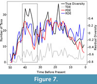 Therefore, phylogenetic diversity estimates are biased towards higher diversity earlier in time, and the Signor Lipps effect will be exaggerated (Lane et al., 2005; see also Figure 7). Moreover, the Spearman’s rank correlation test, based on the rank orders of the values, does not allow one to test whether the magnitude of the diversity changes are reflected accurately. Lane et al. (2005) suggested that the phylogenetic diversity estimate overestimated the magnitude of changes in diversity due to the fact that the relationships of ancestors cannot be fully resolved with their descendants using current phylogenetic methods. Therefore, if both an ancestor and a descendant are sampled, the ancestor will be found to be the sister to its descendant and an incorrect ghost lineage will be inferred, raising the phylogenetic diversity estimate. In several simulations, the phylogenetic diversity estimate was found to be higher than the true diversity in some time bins, even after a sampling filter was applied (Figure 7).

The residual diversity estimate may also be afflicted by problems not identified by the Spearman’s Rank correlation coefficient, such as the Lagerstätten effect. A formation with exceptional preservation will not only raise the diversity estimate of a particular time bin (Raup, 1972), but will also violate the linear relationship between the sampling proxy and inferred diversity; a single formation will produce a lot more species than the others. Thus, Largestätten raise both the taxic and residual diversity estimates. This is observed in Mesozoic birds; despite using the residual diversity estimate to correct for sampling bias, Brocklehurst et al. (2012) still observed peaks in diversity coinciding with Jurassic and Cretaceous areas of exceptional preservation.

In short, all diversity estimates have potential pitfalls. Although the phylogenetic diversity estimate performs best under simulation, there are occasions where its performance is reduced, such as during mass extinctions. The residual diversity estimate does, in certain implementations, perform better than the raw data, and so its use should not be discouraged. Rather, when one is attempting to infer palaeodiversity estimates, one should use multiple methods and compare the results, as has been suggested in recent studies (e.g., Brocklehurst et al., 2013; Fröbisch, 2013; Walther and Fröbisch, 2013; Dunhill et al., 2014). Where disagreement occurs, the strengths and weaknesses of each method may be examined, allowing workers to converge on a true evolutionary history.

Model Limitations and Potential for Further Analyses

This simulation obviously represents an extreme simplification of the sampling biases affecting the fossil record, and is, therefore, only an approximation of the true processes underlying these issues. A model can never fully realise the complexity of the biases that palaeontologists have inflicted on the fossil record. Nevertheless this should not be taken to indicate that this study has no bearing on the real world. Rather it should be taken to represent the minimum set of conditions under which a method should be able to perform. If a method cannot perform under these conditions, then it is unlikely to work well under the more complicated conditions found in the real world. Further simulations can provide more parameters to more closely represent evolution and sampling heterogeneity.

The most obvious limitation is the random nature of sampling. While this model represents the most detailed attempt to simulate sampling, sampling is still treated as a random process; each formation and each locality has the same probability of being sampled as all others in all time bins. As such, sampling variation will be a random walk. In the real world, sampling is strongly heterogeneous; certain countries, continents and formations are sampled considerably more thoroughly than others, either due to historical factors, ease of access or interest of researchers (Benton et al., 2011; Dunhill et al., 2013). It would be interesting to observe the results when different areas are assigned different sampling probabilities; it is possible that the Smith and McGowan method, which assumes a linear relationship between sampling and observed diversity, would perform less well when sampling is heterogeneous. One could also incorporate Largerstätten (areas of exceptional preservation) as single formations where the taphonomic filter is less severe.

Of course this does not fully represent the vagaries surrounding heterogeneity of worker effort. One factor that is probably impossible to represent in a simulation is the definition of formations; there are far too many complicating factors. Formation definitions may incorporate different sedimentation environments and rates, global location, age and the uncertainty that surrounds dating. As has been discussed, they can be hugely arbitrary and variable in their size, and it would be difficult to model effectively all the factors used in their definition.

Finally, one must consider the parameters of the birth-death-dispersal model. In this simulation dispersal is entirely free; any taxon can disperse from any region to any other. Since faunal provinciality has been shown to be a potentially important factor affecting the residual diversity estimate, a more accurate representation of dispersal would be of relevance to the performance of these methods.

No sampling model is a perfect representation of the biases affecting the fossil record. Nevertheless such models are important in identifying the limitations and assumptions of methods. This study has identified a number of considerations that need to be taken into account when performing analyses of palaeodiversity and has potential to act as a starting point for more detailed analyses.

ACKNOWLEDGEMENTS

I would like to thank J. Frӧbisch for helpful comments on early drafts of the manuscript. The reviews of M. Benton and A. Dunhill also greatly improved the manuscript. G. Lloyd and J. Renaudie offered assistance with coding in R. This study was financially supported by a Sofja Kovalevskaja Award to Professor J. Fröbisch of the Museum für Naturkunde, which is awarded by the Alexander von Humboldt Foundation and donated by the German Federal Ministry for Education and Research.

REFERENCES

Alroy, J. 2010a. Fair sampling of taxonomic richness and unbiased estimation of origination and extinction, p. 1211-1235. In Alroy, J. and Hunt, G. (eds.), Quantitative Methods in Paleobiology. Paleontological Society, Boulder.

Alroy, J. 2010b. Geographical, environmental and intrinsic biotic controls on Phanerozoic marine diversification. Palaeontology, 53:1211-1235.

Alroy, J., Aberhan, M., Bottjer, D.J., Foote, M., Fursich, F.T., Harries, P.J., Hendz, A.J.W., Holland, S.M., Ivanz, L.C., Kiessling, W., Kosnik, M.A., Marshall, C.R., McGowan, A.J., Miller, A.I., Olszewski, T.D., Patzkowsky, M.E., Peters, S.E., Villier, L., Wagner, P.J., Bonuso, N., Borkow, P.S., Brenneis, B., Clapham, M.E., Fall, L.M., Ferguson, C.A., Hanson, V.L., Krug, A.Z., Layou, K.M., Leckey, E.H., Nurnberg, S., Powers, C.M., Sessa, J.A., Simpson, C., Tomasovych, A., and Visaggi, C.C. 2008. Phanerozoic trends in the global diversity of marine invertebrates. Science, 321:97-100.

Alroy, J., Marshall, C.R., Bambach, R.K., Bezuko, K., Foote, M., Fursich, F.T., Hansen, T.A., Holland, S.M., Ivany, L., Jablonski, D., Jacobs, D.K., Jones, D.C., Kosnik, M.A., Lidgard, S., Low, S., Miller, A.I., Novack-Gottshall, P.M., Olszewski, T.D., Patzkowsky, M.E., Raup, D.M., Roy, K., Sepkoski, J.J.J., Sommers, M.G., Wagner, P.J., and Webber, A. 2001. Estimates of sampling standardization on estimates of Phanerozoic marine diversification. Proceedings of the National Academy of Sciences , 98:6261-6266.

Bapst, D.W. 2012. Paleotree: an R package for paleontological and phylogenetic analyses of evolution. Methods in Ecology and Evolution, 3:803-803.

Bapst, D.W. 2013. When can clades be potentially resolved with morphology? PlosOne , 8:e62312.

Barrett, P.M., McGowan, A.J., and Page, V. 2009. Dinosaur diversity and the rock record. Proceedings of the Royal Society B, 276:2667-2674.

Benson, R.B.J., Butler, R.J., Lindgren, J., and Smith, A.S. 2010. Palaeodiversity of Mesozoic marine reptiles: mass extinctions and temporal heterogeneity in geologic megabiases affecting vertebrates. Proceedings of the Royal Society B, 277:829-834.

Benson, R.B.J. and Upchurch, P. 2013. Diversity trends in the establishment of terrestrial vertebrate ecosystems: interactions between spatial and temporal sampling biases. Geology, 41:43-46.

Benton, M.J. 2012. No gap in the Middle Permian record of terrestrial vertebrates. Geology, 40:339-342.

Benton, M.J. 2015. Palaeodiversity and formation counts: redundancy or bias? Palaeontology. doi: 10.1111/pala.12191

Benton, M.J., Dunhill, A.M., Lloyd, G.T., and Marx, F.G. 2011. Assessing the quality of the fossil record: insights from vertebrates, p. 63-94. In McGowan, A.J. and Smith, A.B. (eds.), Comparing the Geological and Fossil Records: Implications for Biodiversity Studies. Geological Society Special Publications, London.

Benton, M.J., Ruta, M., Dunhill, A.M., and Sakamoto, M. 2013. The first half of tetrapod evolution, sampling porxies and fossil record quality. Palaeogeography, Palaeoclimatology, Palaeoecology, 372:18-41.

Brocklehurst, N., Kammerer, C.F., and Fröbisch, J. 2013. The early evolution of synapsids and the influence of sampling on their fossil record. Paleobiology, 39:470-490.

Brocklehurst, N., Upchurch, P., Mannion, P.D., and O'Connor, J. 2012. The completeness of the fossil record of Mesozoic bird: implications for early avian evolution. PlosOne, 7:e39056.

Butler, R.J., Barrett, P.M., Nowbath, S., and Upchurch, P. 2009. Estimating the effects of the rock record on pterosaur diversity patterns: implications for hypotheses of bird/pterosaur competitive replacement. Paleobiology, 35:432-446.

Butler, R.J., Benson, R.B.J., Carrano, W.T., Mannion, P.D., and Upchurch, P. 2011. Sea level, dinosaur diversity and sampling: investigating the 'common cause' hypothesis in the terrestrial realm. Proceedings of the Royal Society B, 278:1165-1170.

Chao, A., Colwell, R.K., Lin, C.-W., and Gotelli, N.J. 2009. Sufficient sampling for asymptotic minimum species richness estimators. Ecology, 90:1125-1133.

Crampton, J.S., Beu, A.G., Cooper, R.A., Jones, C.M., Marshall, B., and Maxwell, P.A. 2003. Estimating the rock volume bias in paleobiodiversity studies. Science, 301:358-360.

Dunhill, A.M. 2012. Problems with using rock outcrop area as a paleontological sampling proxy: rock outcrop and exposure area compared with coastal proximity, topography, land use and lithology. Paleobiology, 38:126-143.

Dunhill, A.M., Benton, M.J., Newell, A.J., and Twitchett, R.J. 2013. Completeness of the fossil record and the validity of sampling proxies: a case study from the Triassic of England and Wales. Journal of the Geological Society, 170:291-300.

Dunhill, A.M., Hannisdal, B., and Benton, M.J. 2014. Disentangling rock record bias and common-cause from redundancy in the British fossil record. Nature Communication , 5:4818.

Fröbisch, J. 2008. Global taxonomic diversity of anomodonts (Tetrapoda, Therapsida) and the terrestrial rock record across the Permian-Triassic boundary. PlosOne, 3:e3733.

Fröbisch, J. 2013. Vertebrate diversity across the end-Permian mass extinction - separating biological and geological signals. Palaeogeography, Palaeoclimatology, Palaeoecology, 372:50-61.

Fröbisch, J. 2014. Synapsid diversity and the rock record in the Permian-Triassic Beaufort Group (Karoo Supergroup), South Africa, p. 305-319. In Kammerer, C.F., Angielczyk, K.D., and Fröbisch, J. (eds.), Early Evolutionary History of the Synapsida. Springer, New York.

Lane, A., Janis, C.M., and Sepkoski, J.J.J. 2005. Estimating paleodiversities: a test of the taxic and phylogenetic methods. Paleobiology, 31:21-34.

Lloyd, G.T. 2012. A refined modelling approach to assess the influence of sampling on palaeobiodiversity curves: new support for declining Cretaceous dinosaur richness. Biology Letters, 8:123-126.

Lloyd, G.T., Davis, K.E., Pisani, D., Tarver, J.E., Ruta, M., Sakamoto, M., Hone, D.W.E., Jennings, R., and Benton, M.J. 2008. Dinosaurs and the Cretaceous Terrestrial Revolution. Proceedings of the Royal Society B, 275:2483-2490.

Mannion, P.D., Upchurch, P., Carrano, W.T., and Barrett, P.M. 2011. Testing the effect of the rock record on diversity: a multidisciplinary approach to elucidating the generic richeness of sauropodomorph dinosaurs through time. Biological Reviews, 86:157-181.

Miller, A.I. and Foote, M. 1996. Calibrating the Ordovician radiation of marine life: implications for Phanerozoic diversity trends. Paleobiology, 22:304-309.

Norrell, M. 1992. Taxic origin and temporal diversity: the effect of phylogeny, p. 89-118. In Novacek, M. and Wheeler, Q. (eds.), Extinction and Phylogeny. Columbia University Press, New York.

Pearson, M., Benson, R.B.J., Upchurch, P., Fröbisch, J., and Kammerer, C.F. 2013. Reconstructing the diversity of early terrestrial herbivorous tetrapods. Palaeogeography, Palaeoclimatology, Palaeoecology, 372:41-49.

Peters, S.E. 2006. Macrostratigraphy of North America. Journal of Geology, 114:391-412.

Peters, S.E. and Foote, M. 2001. Biodiversity in the Phanerozoic: a reinterpretation. Paleobiology, 27:583-601.

Peters, S.E. and Heim, N.A. 2010. The geological completeness of paleontological sampling in North America. Paleobiology, 36:61-79.

Preston, F.W. 1962. The canonical distribution of commonness and rarity: Part I. Ecology, 43:185-215.

Raup, D.M. 1972. Taxonomic diversity during the Phanerozoic. Science, 177:1065-1071.

Ruta, M., Cisneros, J.C., Liebrecht, T., Tsuji, L.A., and Müller, J. 2011. Amniotes through major biologícal crises: faunal turnover among parareptiles and the end-Permian mass extinction. Palaeontology, 54:1117-1137.

Sanders, H.L. 1968. Marine benthic diversity: a comparative study. The American Naturalist, 102:243-282.

Schliep, K. 2011. Phangorn: Phylogenetic analysis in R. Bioinformatics, 27:592-593.

Smith, A.B. 1994. Systematics and the Fossil Record: Documenting Evolutionary Patterns. Blackwell, London.

Smith, A.B. 2001. Large scale heterogeneity of the fossil record: implications for Phanerozoic biodiversity studies. Proceedings of the Royal Society B, 356:351-367.

Smith, A.B. and McGowan, A.J. 2007. The shape of the Phanerozoic palaeodiversity curve: how much can be predicted from the sedimentary rock record of western Europe. Palaeontology, 50:765-774.

Smith, A.B., and McGowan, A.J. 2008. Temporal patterns of barren intervals in the Phanerozoic. Paleobiology, 34:155-161.

Smith, A.B., Lloyd, G.T., and McGowan, A.J. 2012. Phanerozoic marine diversity: rock record modelling provides an independent test of large-scale trends. Proceedings of the Royal Society B, 279:4489-4495.

Smith, E.P., Stewart, P., and Cairns, J. 1985. Similarities between rarefaction methods. Hydrobiologia, 120:167-170.

Upchurch, P. and Barrett, P.M. 2005. Phyogenetic and taxic perspectives on sauropod diversity, p. 104-124. In Rogers, K.C. and Wilson, J.A. (eds.), The Sauropods: Evolution and Palaeobiology. University of California Press, Berkley and Los Angeles, California.

Wall, P., Ivany, L., and Wilkinson, B. 2009. Revisiting Raup: exploring the influence of outcrop area on diversity in light of modern sample standardization techniques. Paleobiology, 35:146-167.

Walther, M. and Fröbisch, J. 2013. The quality of the fossil record of anomodonts. Comptes Rendus Pelevol, 12:495-504.

Zhang, H. and Stern, H. 2009. Sample size calculation for finding unseen species. Bayesian Analysis, 4:763-792.