

 Testing the impact of two key scan parameters on the quality and repeatability of measurements from CT scan data
Article number: 23(1):a07
https://doi.org/10.26879/942
Copyright Paleontological Society, March 2020
Author biographies
Plain-language and multi-lingual abstracts
PDF version
Submission: 9 November 2018. Acceptance: 5 February 2020.
ABSTRACT
Computed tomographic (CT) scanning is becoming a popular research tool across earth and life sciences. However, despite its prominence, there have not been systematic investigations into how CT scan parameters affect data quality and reproducibility. Here we conduct two sets of trials to test how exposure time, the number of x-ray radiographs averaged per view, and overall scan time affect the quality of CT scan data, assessed using signal and contrast to noise ratios and the repeatability of measurements derived from these data, in this case the calculated volume of pteropod shells. We find that contrast to noise ratio and calculated shell volume increase and the variability in shell volume measurements decrease with increasing overall scan time. However, the benefits of increased overall scan time diminish considerably at scan times of 50 minutes or more. Furthermore, as overall scan time increases, scans are at greater risk of being affected by sample movement, which can make the data unusable. By balancing exposure time and the number of x-ray radiographs averaged per view, the image quality in a 50-minute scan can be comparable to, or better than, that collected in a 75-minute scan. By selecting a 50-minute rather than a 75-minute scan, data collection can be increased by between 66 and 75%, maximizing both the quantity and quality of CT data collected.
Rosie L. Oakes. Academy of Natural Sciences of Drexel University, Philadelphia, Pennsylvania, USA. roakes@drexel.edu
Morgan Hill Chase. American Museum of Natural History, New York, New York, USA. mchase@amnh.org
Mark E. Siddall. American Museum of Natural History, New York, New York, USA. siddall@amnh.org
Jocelyn A. Sessa. Academy of Natural Sciences of Drexel University, Philadelphia, Pennsylvania, USA. jsessa@drexel.edu
Keywords: CT scanning; computed tomography; scan quality; pteropod
Final citation: Oakes, Rosie L., Hill Chase, Morgan, Siddall, Mark E., and Sessa, Jocelyn A. 2020. Testing the impact of two key scan parameters on the quality and repeatability of measurements from CT scan data. Palaeontologia Electronica, 23(1):a07. https://doi.org/10.26879/942
palaeo-electronica.org/content/2020/2923-investigating-ct-scan-quality
Copyright: March 2020 Society of Vertebrate Paleontology.
This is an open access article distributed under the terms of the Creative Commons Attribution License,
which permits unrestricted use, distribution, and reproduction in any medium, provided the original author and source are credited.
creativecommons.org/licenses/by/4.0
INTRODUCTION
The use of computed tomographic (CT) scanning in science and industry has grown rapidly since its inception over 45 years ago (Hounsfield, 1973). Although the first applications of this technique were restricted to the medical field, CT scanning technology was soon being applied to image specimens from geology, paleontology, and anthropology (Arnold et al., 1983; Wind, 1984; Feldkamp et al., 1989). The non-destructive nature of this technique is invaluable for imaging scientifically important and delicate specimens that could not easily be loaned for study, or studied without destroying the specimen (Sutton, 2008; Garwood et al., 2010; Cunningham et al., 2014; Landman, 2018). Consequently, CT scanning has been used to investigate a wide range of specimens, from fossilized plankton and planktonic snails (Görög et al., 2012; Janssen et al., 2016; Peck et al., 2018) to fossil frogs (Matthews and du Plessis, 2017; Xing et al., 2018), ammonites (Hoffmann et al., 2014; Inoue and Kondo, 2016), flying reptiles (Witmer et al., 2003), mummies (Hoffman et al., 2002; Petrella et al., 2016), and meteorites (Jenniskens et al., 2012). Advances in staining techniques enable density differences to be artificially created so that soft-bodied organisms, such as leeches, can be imaged and described using CT scanning (Metscher, 2009; Cunningham et al., 2014; Tessler et al., 2016). Studies of soft bodied organisms were previously accomplished via histological sectioning and imaging on a light microscope, which are destructive, error-prone, and time consuming techniques (Lauridsen et al., 2011).
Data that are yielded from CT scans can be shared more easily than the delicate specimens that they are derived from, and 3D-datasets can be uploaded to online servers (e.g., Dryad, datadryad.org; MorphoSource, morphosource.org, Phenome 10K, phenome10k.org) to supplement museum collections and be used by other researchers (Davies et al., 2017). Furthermore, shapes files can be generated from these data and 3D printed for use in research, education, and outreach (e.g., https://tinyurl.com/3Dprintingplankton, Rahman et al., 2012; Lautenschlager and Rücklin, 2014).
Despite the many advantages of CT scanning, there are drawbacks, primarily the cost and the time it takes to scan a specimen. The cost of scan time varies widely: for example, the University of Texas High-Resolution x-ray Computed Tomography Facility (UTCT) charges $125/ hour for academic projects and $297/ hour for commercial work, the Florida Museum of Natural History charges $52.50/ hour for external academic projects and $300/ hour for external commercial work, and the University of Arkansas charges $120/ hour for academic projects and $175/ hour for commercial work (all prices as of October 2019). Even at institutions that offer time to their employees free of charge, such as the Natural History Museum in London (NHM) and the American Museum of Natural History in New York (AMNH), user demand can limit the time available for scanning. For example, at the AMNH, time for curators is limited to two days a month, which is booked three months in advance (AMNH MIF User Policy, available online). At NHM, researchers submit proposals for CT time on a quarterly basis, with each project being awarded a maximum of one week of scan time per quarter (NHM x-ray micro-CT lab user policy, V. Fernandez, personal communication). Because of costly scan time and/or high user demand, scientists are frequently restricted by the amount of scan time available to them. With limited time comes limited data, forcing researchers to decide whether to collect a lower number of high-quality scans, or a higher number of low-quality scans.
Introduction to X-ray CT Scanning
Before discussing how changing scan parameters impacts the quality of a CT scan, we provide a brief overview of the physics behind the creation of x-rays, their interaction with the material of interest, their detection and collection, and how x-ray radiographs are reconstructed. A more detailed summary can be found in Sutton et al. (2014). Throughout the text, ‘x-rays’ is used to refer to the electromagnetic radiation produced by photons, and ‘x-ray radiograph’ is used to refer to the generated images.
A CT scan is created by reconstructing a series of x-ray radiographs taken at hundreds or thousands of angles, or projections, around an object of interest. The density and chemical composition of the object will determine how much energy the x-rays lose during their path from the x-ray tube to the detector. Following scanning, x-ray radiographs are reconstructed using the FDK (Feldkamp, Davis, and Kress) filtered back projection algorithm (Feldkamp et al., 1984) to create a 3D volume rendering of the object. This 3D rendering can be used to investigate the internal and external structure of the object, as well as the density of the material.
X-ray generation. X-rays are generated in the x-ray tube by passing a current through a tungsten filament (cathode), which causes it to increase in temperature and release electrons. These electrons are accelerated through a vacuum to collide with the anode, or target, decelerating the electrons and producing heat and x-rays. The energy-profile of the resulting x-rays (keV) is determined by the accelerating voltage between the cathode and the anode, and the material of the anode target (Sutton et al. 2014). The current passing through the filament determines the number of photons produced by the x-ray tube, known as the x-ray intensity. X-ray tube power is a measure of the energy that the electron beam has, which is a combination of the x-ray energy (voltage) and x-ray intensity (current). In this experiment we used a diamond-tungsten target, where the surface of a diamond plate is coated with a thin layer of tungsten. The x-rays are produced from the tungsten target and the diamond disperses the heat, enabling a smaller focal spot size to be maintained at higher power, which is necessary for imaging the specimens of interest in this study as they are typically 2 mm or less in diameter. Molybdenum and tungsten targets are also commonly used in natural science research.
Setting up the scan. Throughout the course of the scan, x-ray radiographs are taken at 360° around an object, with each view known as a projection. The number of projections necessary is calculated using Equation 1 (Kak and Slaney, 2001; du Plessis et al., 2017):
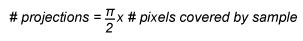 (Eq. 1)
The object must be mounted so that its longest axis is vertical, limiting the path length that x-rays have to travel through the object, and reducing the potential of developing scan artefacts, which are discrepancies between the measured and true attenuation properties of the object of interest (Barrett and Keat, 2004). It is crucial that the specimen does not move during the scan as this can lead to the formation of scan artefacts, or, in the case of too much movement, a scan which cannot be reconstructed and is therefore unusable (Ketcham and Carlson, 2001).
X-ray interaction with object. X-rays interact with matter via three mechanisms: the photoelectric effect, Compton scattering, and Rayleigh scattering (Sutton et al., 2014). The photoelectric effect occurs when the energy of the x-ray is slightly higher than the binding energy of the electrons in the object of interest. In this case, the attenuation of the x-ray is strongly affected by the chemical composition of the object. Compton scattering occurs when the energy of the x-ray is much higher than the binding energy of the electrons in the object being scanned. In this case, x-ray attenuation is more affected by the density of the object (Sutton et al., 2014). Rayleigh scattering occurs at very low energies (i.e., 1-50 kV): when the x-ray interacts with an atom in the object of interest, the x-ray wavelength remains constant but the direction of the photon is deflected. When x-rays interact with low density material, for example in the air surrounding the object being scanned, the x-rays will undergo very little attenuation.
X-ray detection. After passing through the object of interest, the energy of the resulting x-rays is recorded using a detector, a panel containing a two-dimensional array of pixels. Most micro-CT scanners, including the one used in this study, use solid state detectors with a top scintillator layer. The scintillator layer coverts the x-rays into visible light: a higher flux of photons reaching the detector will result in higher values being recorded. The solid-state pixels underneath the scintillator layer convert the light into an electric current proportional to the light intensity at each pixel. An analog-to-digital converter translates the current intensity to a digital numeric value. These numeric values are displayed as greyscale values on a monitor. The number of pixels on the detector and the maximum diameter of the object or region of interest constrain the smallest voxel size that can be achieved during a scan. For example, in this investigation we used a 1000 x 1000-pixel detector, so the minimum voxel size possible is 1/1000th of the diameter of our object of interest.
Data reconstruction. During reconstruction, the two-dimensional projections are reconstructed to make a three-dimensional dataset. The software used in this study (phoenix datos|x 2.1) applies the FDK filtered back projection reconstruction algorithm (Feldkamp et al., 1984), which determines the incremental contribution of each projection to the final reconstructed density. Each projection is 1000 x 1000 pixels so the reconstructed data is a three-dimensional 1000 x 1000 x 1000-pixel dataset, where each three-dimensional pixel is known as a voxel. In most machines, this process is largely automated by the reconstruction software. The user needs to provide the center of rotation as an input value for the reconstruction mathematics; this value can either be entered manually, or calculated using the reconstruction software (Kak and Slaney 2001). If the specimen has moved too much during the scan, pixels cannot be tracked across successive projections and reconstruction will fail, i.e., the collected data are unusable.
When CT data are reconstructed, the information about a three-dimensional, curved object is transposed onto a 3D grid. These gridded data therefore have to be interpolated to calculate the ‘true surface’ of the object. The threshold for which pixels are counted as shell and which as background can be calculated using computer software or can be adjusted manually by the user. This threshold will determine how all the pixels in the dataset are classified (i.e., as shell or as background material, which is typically air). In this study we used VGSTUDIO MAX v. 3.1 to determine material thresholds (see methods section for further details).
Scan quality. The utility of a scan for scientific research depends on the ability to resolve and differentiate the features of interest. If the specimen is formed of multiple materials with a range of densities, the x-rays will be attenuated differently when interacting with these materials resulting in each material being represented by a unique range of greyscale values in the reconstructed CT dataset. When studying the impact of ocean acidification on pteropod shells, for example, the shell material, rather than the internal soft parts of the organism, are the focus (e.g., Peck et al., 2018). In order for these phases to be separated digitally, the grey scale values of the pixels representing the air, organics, and shell need to be sufficiently different.
Much like in a photographic film, if there is not enough signal reaching the detector, comparable to light hitting the film, the image will have low contrast and the different phases cannot be separated. Conversely, if there is too much signal reaching the detector, the resulting x-ray radiographs will be oversaturated, making it impossible to separate the different phases. In both of these end-members, there will be too much overlap in the grey scale ranges of each material, limiting separation and therefore causing non-shell pixels to be falsely classified as shell material, or vice-versa. This will introduce a source of error into any measurements made on the dataset. When setting up a scan, the aim is therefore to maximize the span of the grey scale values in the dataset, without hitting the extremes (pure black and pure white), which represent a total lack of signal, or overexposure, respectively.
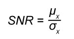
The quality of CT scans can be quantified using metrics such as the signal-to-noise ratio (SNR) and the contrast-to-noise ratio (CNR) (e.g., Bhosale et al., 2016; Kraemer et al., 2015). The SNR is a measure of the signal relative to the variation:
 (Eq. 2)
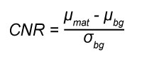
where µ is mean, σ is standard deviation, and x is the material of interest. The separation of the material of interest from the background is assessed using the CNR:
 (Eq. 3)
where mat is the material of interest, which in this study is the shell material, and bg is the background material, which in most cases, including in this study, is air.
Scan artefacts. The quality of CT scan data can be negatively impacted by artefacts that are introduced into the dataset during scanning but can only be observed after the data have been reconstructed. The most basic artefact, which will be found in every scan, is noise, where a pixel from a homogenous material (e.g., air) has a pixel value that differs from the rest of the pixels of that same material, resulting in a mottled appearance.
Artefacts can also be introduced by selecting too few projections (Eq.1), which causes dark and light streaks, or streak artefacts, to appear parallel or sub-parallel to the edges of the scanned object. Ring artefacts, which appear as circular light and dark rings that are worse in the center of the projection, are caused by variability or malfunction of the detector elements (i.e., pixels in the detector panel). Motion artefacts are caused by the movement of the sample or a shift in the beam during the scan (i.e., beam shift) and appear as streaks, or false broken edges of the scanned object. Beam hardening artefacts are common in dense samples where low energy x-rays are preferentially attenuated relative to high energy x-rays. Partial averaging artefacts appear as a blurring of the edges of the scanned object, caused by the fact that the intensity of any voxel represents the mean energy of the x-rays hitting that voxel, and hence may be an average of two media (i.e., air and shell). The best way to minimize scan artefacts is during set-up, although there are an increasing number of computational-based methods that reduce scan artefacts in cases where changing scan parameters is not an option (e.g., Tang and Tang, 2012).
Overall scan time. There is a perception that a longer scan will yield better data, but overall scan time and data quality are influenced by a wide range of factors. Scan time is influenced by three factors: the numbers of projections collected around the specimen; the exposure time of each x-ray radiograph, and the numbers of x-ray radiographs taken and averaged per view. Scan quality, or the ability to separate different materials, is influenced by these factors, as well as the energy of the x-rays, the voxel size, and the quality of the detector.
Investigations led by the non-destructive testing and inspection industry have researched the impacts of varying some of these parameters on scan quality (e.g., Wenig and Kasperl, 2006), however, these studies are usually designed to test industrial equipment that has very different densities and are more homogenous than biologic and geologic specimens. Here we conduct a series of scans to test how two key CT scan parameters: exposure time, and the number of x-ray radiographs averaged per view, affect the quality of the acquired CT scan data assessed using SNR, CNR, and the reproducibility of shell volume measurements. The results of this study can be used to determine how to balance scan quality and cost, and maximize research money and time, while collecting research-quality CT scan data.
CT Scanning Thecosome Pteropods
The scans in this study are conducted on the shells of thecosome pteropods from the species Limacina retroversa. Pteropods are a group of planktonic molluscs that are predicted to be among the first organisms to be impacted by ocean acidification (Orr et al., 2005; Bednaršek et al., 2017), the term for the changes in ocean chemistry caused by rising atmospheric carbon dioxide concentrations (Caldeira and Wickett, 2003). Pteropods form their shells from aragonite, a more soluble form of calcium carbonate (Mucci, 1983), which is predicted to become chemically unstable in the Arctic Ocean within the next few decades (Steinacher et al., 2009) and in the Southern Ocean seasonally by 2035 and nearly permanently by 2100 (McNeil and Matear, 2008; Hauri et al., 2015). There is, therefore, an interest in monitoring pteropods over the coming decades (Bednaršek et al., 2014, 2017). One aspect of this monitoring could involve using CT scanning to measure the shell thickness of pteropods and assessing whether their ability to build and maintain their shells is affected by changes in ocean chemistry (e.g., Howes et al., 2017; Peck et al., 2018; Oakes et al., 2019a). Aside from their scientific interest, pteropod shells are ideal specimens to use for a CT methodology study because their overall size (< 1 mm) and the thickness of their shells (~10 µm) pushes the limits of most modern micro-CT scanners.
MATERIALS AND METHODS
Here we investigate the precision of CT-based measurements by: systematically varying scan parameters to address how different scan settings affect scan quality and quantitative measurements of pteropod shell volume; and repeating scans at the same settings to test the reproducibility of these measurements. Ideally, we would have run all trials on a single specimen but, unfortunately, the shell we began these experiments with broke during handling before the full matrix of scans could be completed (Table 1). Therefore, the experiment was split into two parts: the scan parameter experiment, and the repeatability experiment, with each experiment conducted on a different shell.
Sample Collection
For both experiments, shells of the pteropod Limacina retroversa collected from the Scotia Sea were scanned. The sample that contained the specimen used for the scan parameter experiment was collected on 11th January 2013 on cruise JR274 to the Scotia Sea (-56.467 °N, -57.426 °E). The sample that contained the specimen used for the repeatability experiment was collected on December 8, 2015, on cruise JR15002 to the Scotia Sea (-52.812 °N, -40.112 °E). Both samples were collected using a British Antarctic Survey motion compensated bongo net hauled from 200 m to 0 m. Following the methodology recommended by Oakes et al. (2019b), on collection, specimens were picked with a wide mouthed plastic pipette and terminated by rinsing with deionized water buffered with ammonium hydroxide, and air dried overnight.
CT Scan Methodology
For CT scanning, specimens were mounted onto a 3 mm diameter, 15 cm long glass rod using a small piece of carbon tape and scanned on a GE PHOENIX v|tome|x s with a 180 kV x-ray tube with a diamond target and a DXR250 detector at the Microscopy and Imaging Facility (MIF) at the AMNH. Scans were run at 70 kV and 210 µA in focus mode 1. The voltage, current, and focus settings are based on the settings we have used to scan pteropods in previous studies (e.g., Oakes et al., 2019a) but we acknowledge that varying these parameters could also impact scan quality and therefore could be investigated in another study. Detector sensitivity was set to 2, meaning that the light signal generated when the x-rays hit the scintillator on the detector was multiplied by two as it was converted from analog to digital. This increases the strength of both the signal and the noise in the generated dataset. Specimens were rotated through 360° during the scan and x-ray radiographs were taken at 1500 projections (calculated using Eq. 1).
The exposure time and the number of x-ray radiographs averaged per view were varied among scan trials; these parameters contribute to the overall scan time, which thus varies depending on trial parameters. For example, a 50-minute scan could be reached with an exposure time of 333 ms and five x-ray radiographs averaged per view, an exposure time of 400 ms and four x-ray radiographs averaged per view, or an exposure time of 500 ms and three x-ray radiographs averaged per view (see Table 1 for details). In the scan parameter experiment, we performed 11 trials to assess how varying exposure time, from 200 ms to 500 ms, and varying the number of x-ray radiographs averaged per view, from two through five radiographs per view, affected the quality of the CT data (Table 1).
 The voxel (i.e., 3D pixel) size was kept constant throughout all scans except one where it was doubled to test the impact of voxel size on calculated shell volume. This is noted in Table 1, and that data point is excluded from Figure 1A-C to reduce the number of variables presented. In the repeatability experiment, we performed 16 trials, repeating measurements at 333 ms, 400 ms, and 500 ms exposure times with three, four, and five x-ray radiographs averaged per view to assess the precision of the CT scan data. In both experiments, shells were not re-mounted between scans and trial order was randomized.
CT Data Reconstruction and Segmentation
Scan data were reconstructed using the GE software phoenix datos|x 2.1 and analyzed in the software VGSTUDIO MAX v.3.1. The thresholds for which pixels were counted as shell, organic material, and air, were calculated using a surface determination module within VGSTUDIO MAX v.3.1. We tested the effect of 10 surface determination modules on the shell volume calculated from three scans (see Appendix 1, Table A1, and Figures A1.1 and A1.2, for more details. Data are available in Appendix 2 for more details). Based on these trials, all the analyses presented here use the automatic surface determination module where the differentiation between material and background is calculated using the following equation:
 (Eq. 4)
where the ‘material’ and ‘air’ values are selected by picking the two most prominent peaks on the grey scale distribution histogram. This is also called the iso50 method and gives sub-voxel precise surface determination (VGSTUDIO MAX, 2018).
Assessment of CT-scan Quality
The quality of the CT-scan data in this study was assessed in two ways: 1) conducting traditional CT scan quality assessments of SNR of the background material (air), SNR of the material, in this case shell, and CNR (Equations 2, 3); and 2) measuring the volume of the pteropod calculated from the scan data to assess the repeatability of measurements at different scan settings. Shell volume was chosen as a comparative tool because it is sensitive to changes in scan quality, i.e., it is likely to be affected by both noise and low contrast between the different materials (shell, body, and air). Measuring pteropod shell volume in combination with shell size has practical applications as it could be used as a metric for monitoring the response of pteropods to ocean acidification in the future (e.g., Howes et al., 2017; Oakes et al., 2019a).
Quality assessment method 1-SNR and CNR. The mean and standard deviation of grey scale values were measured on the reconstructed datasets in VGSTUDIO MAX v.3.1. The background values were collected from a representative cube of air, which is the background material in these scans. The shell material was separated from the organic material and air using the automatic surface determination module (outlined above). A region of interest (ROI) was created from the shell surface so that just the grey values of the shell material could be analyzed. The mean and standard deviation values for both the background and the shell material were measured using the grey value analysis tool in VGSTUDIO MAX v.3.1.
Quality assessment method 2-pteropod shell volume. Measured shell volume was used as a metric to compare between the different scans. Shell volume was calculated using the object properties module in VGSTUDIO MAX v. 3.1. This module calculates the number of voxels within the selected ‘shell’ grey scale range calculated by the selected surface determination method, and multiplies that by the voxel size, giving the total volume of data with ‘shell’ grey scale values.
Beam shift analysis. One component that factors into the creation of scan artefacts is beam shift, the apparent movement of the specimen caused by the heating of the tube during scanning. Beam shift was quantified by measuring the ‘scaling’ factor applied during reconstruction of the x-ray radiographs in phoenix datos|x 2.1; this scaling factor is recorded in the reconstruction files (.pca). The scaling factor represents the size of the shell in the final x-ray radiograph relative to the first x-ray radiograph. As the shell does not change size during the scan, all scaling can be attributed to beam shift.
Statistical Methods
All statistical analyses were conducted in R Studio v. 3.6.0 (R Core Team, 2019). CNR and SNR data are plotted as box and whisker plots. As there were not an equal number of trials run at all exposure times, x-ray radiograph averages, or scan times, sample sizes for statistical tests were unequal and the distributions were non-normal. We therefore used the Kolmogorov-Smirnov Test (K-S test) to test for significant differences between trial groups. For the scan parameter and repeatability experiments, the average and standard deviation of calculated shell volume measurements were used to compare between different trial settings (Table 2).
RESULTS
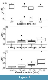
 The quality of the CT scans, assessed using signal-to-noise and contrast-to-noise ratios (SNR, CNR, Figure 1, Figure A2, Figure A3, and Figure A4, Appendix 3), and calculated shell volume (Figure 2, Appendix 4) is affected by scan settings. Figure 1 shows how the CNR is affected by the exposure time, the number of x-ray radiographs averaged per view, and the overall scan time. Increased exposure time has no effect on the CNR (Figure 1A). Background SNR increases with increasing exposure time (Figure A2A), producing scans with a significantly less noisy background at exposure times of 400 ms and greater as compared to those with exposure times of 333 ms or less (K-S test: D = 0.55897; p = 0.02576). However, the material SNR decreases with increased exposure time (Figure A2B), with exposure times of 333 ms and lower producing significantly less noisy scans than those with exposure times of 400 ms and higher (K-S test: D = 0.77949; p = 0.0004223). Increasing the number of x-ray radiographs per view has no significant effect on the CNR (Figure 1B). Background SNR increases with increased number of x-ray radiographs averaged per view, while the material SNR decreases with increased number of x-ray radiographs (Figure A3A, A3B). Increasing the overall scan time increases the CNR, with scans of 50 minutes and longer producing significantly less noisy scans than those of 49 minutes and shorter (K-S test: D = 0.57949, p = 0.01861) (Figure 1C). There is no significant increase in CNR when scan time is increased from 50-69 minutes to 70-89 minutes (K-S test: D = 0.38889, p = 0.7077). Background SNR increases with increasing overall scan time, while material SNR decreases with increasing overall scan time (Figure A4A-A4B).
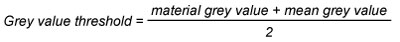
Figure 2 shows how the exposure time, number of x-ray radiographs averaged per view, and the overall scan time affect the calculated volume of the pteropod shell in both the scan parameter experiment (Figure 2A-2C) and the repeatability experiment (Figure 2D-2F). Generally, as exposure time increases, the variability of volume measurements decreases (Figure 2A, 2D). Similarly, as the number of x-ray radiographs averaged per view increases, the variability of volume measurements decreases (Figure 2B, 2E, Table 2).
The volumes calculated in the scan parameter experiment (Figure 2A-2C) converge at exposure times of 400 ms and greater, averages of four or more x-ray radiographs per view, and scan times of 50 minutes and greater. The reproducibility of scans in these ranges were explored further in the repeatability experiment where scans were conducted multiple times within the parameter space of 333 to 500 ms exposure time and three to five x-ray radiographs averaged per view (Figure 2D-2F). The most replicable exposure time was 500 ms per view, with measurement standard deviation of 0.003 mm3. The most replicable number of x-ray radiographs averaged per view was four, where the standard deviation of measurements was 50% lower than when three x-ray radiographs were averaged per view (Figure 2D-2F, Table 2). As overall scan time increases, calculated shell volume increases, and variability of measurements decreases. The benefit of increasing scan time plateaus at overall scan times of 50 minutes or greater, as both the variability in measurements and the calculated shell volume stabilize at this point (Figure 2C, 2F; Table 2).
The impact of the voxel size on calculated shell volume was tested in the scan parameter experiment by performing the longest overall scan (500 ms exposure time, 5 x-ray radiographs averaged per view) at high resolution (1.861 μm3 voxel size), and low resolution (two times the high-resolution voxel size = 3.722 μm3). Calculated shell volumes for the high-resolution scans (voxel size = 1.861 μm3) range between 0.045 and 0.051 mm3 while the low-resolution scan (voxel size = 3.722 μm3) was 0.042 mm3.
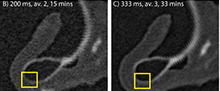
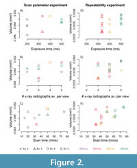
 Scan quality can also be observed visually. Figure 3 shows how a curved object, such as a pteropod shell, is translated onto a grid during data collection. Figure 3B-3E show slices of the pteropod shell from the scan parameter experiment scanned in four different trials, from the shortest overall scan time (200 ms, two x-ray radiographs/ view, 15-minute [Figure 3B]) through intermediate times in Figure 3C-3D, to the longest scan time (500 ms, five x-ray radiographs/ view, 75-minute [Figure 3E]). In the shortest two scans (Figure 3B-3C), the low greyscale contrast between the different materials causes the image to appear fuzzy, blurring the edges of the shell and making it difficult to differentiate the shell (white) from the organic material (dark grey) and the surrounding air (black). At longer scan times (Figure 3D-3E), there is a sharper contrast between the three phases, increasing the certainty of which pixels represent shell material, making the materials easier to separate. These visual observations are in alignment with the CNR measurements, which more than double between the shortest scan (200 ms, two x-ray radiographs/view) and the longest scan (500 ms, five x-ray radiographs per view) (Figure 1C; Table A4).
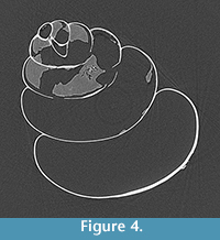
We observe scan artefacts as streaks across the reconstructed CT images, especially at longer scan times (Figure 4). Beam shift, which causes apparent movement of the specimen associated with the heating of the x-ray tube during the scan, was strongly correlated with the time of day, with beam shift reducing through the day (Figure A5A). There was no correlation between beam shift and scan length (Figure A5B).
DISCUSSION
 The contrast to noise ratio and signal to noise ratio of both the background and the shell material, and the calculated shell volume, are influenced by the number of x-ray radiographs averaged per view, the exposure time, and the overall scan time (Figure 1, Figure 2, Figure 3). Calculated shell volume increases, and variability in calculated shell volume decreases, with increasing scan time, up to a point (50 minutes) when the benefit of increasing scan time diminishes as calculated volumes stabilize, the variability in measurements are reduced, and the CNR does not increase significantly.
Generally, scan quality increases with overall scan time (Figure 1C), mainly driven by reduced background noise (Figure A2A, Figure A3A, Figure A4A). The increase in background SNR with an increasing number of x-ray radiographs averaged per view (Figure A2A) is unsurprising, because the noise in the background is random, and averaging an increased number of x-ray radiographs per view will increase the chance that this noise is reduced. However, the material SNR decreases with an increasing number of x-ray radiographs averaged per view (Figure A2B), which implies that the data are noisy, and that this noise is not random. We speculate that the decrease in material SNR may be caused by the thin (8 µm) shell walls and low volume of shell material available to be analyzed for this measurement. We expected to see the SNR of both the material and the background increase with increased exposure time as more signal reached the detector. Although increasing exposure time does have a significant effect on improving background SNR at times of 400 ms and greater, it does not have any effect on the material SNR. This may be because at the current settings used in this experiment (230 µA), signal is not a limiting factor. This warrants future investigation because scanning with high currents could be an effective strategy for decreasing CT scan times.
The increase in calculated shell volume with increased scan time is likely linked to the fact that with more signal reaching the detector, there is more certainty about which pixels should be classified as shell, soft body, and background (Figure 3). This is supported by measurements of CNR, which indicate scans get less noisy with increasing scan time, up to overall scan times of 50 minutes, at which point increasing scan time has diminishing returns (Figure 1C).
The lower calculated shell volume in the low-resolution scan (voxel size 3.722µm3) is likely caused by the partial volume effect, the term for when one voxel has to represent two or more materials (Sutton et al. 2014). In these cases, the voxel is assigned an average grey scale value of the two materials and therefore likely will not fall into the shell material grey scale range, resulting in a lower calculated shell volume.
Generally, CT scans collected at longer overall scan times were more likely to have scan artefacts. The scan artefacts in our data appear as streaking through the reconstructed CT slices (Figure 4). These could be caused by three processes: 1) beam hardening, where the x-ray beam is attenuated less at certain object positions as it passes through less shell material (Boas and Fleischmann, 2012); 2) Compton scattering, where differences in material densities cause scattering at high x-ray energies (Sutton et al., 2014); and/ or 3) movement of either the beam (beam shift) or the specimen during the scan (Barrett and Keat, 2004; Wenig and Kasperl, 2006). Although scan artefacts occur at all settings, there is more signal reaching the detector at longer scan times, and therefore these artefacts become more prominent. The pteropod shells were secured in the same manner for all scans and were not remounted between scans, however, sometimes the vibrations of the machine can cause the shell to move, and statistically, these random movements are more likely to happen at longer overall scan times. Beam shift was measured directly and was found not to be affected by the length of the scan time (Figure A5B). Beam shift decreased through the day (Figure A5A), which reflects the amount of time that the x-ray tube had been in use. Although the effect of beam shift cannot be avoided, it is an interesting source of variability to consider when reconstructing scan data.
The variability of calculated shell volume is reduced at scan times of 50 minutes and greater, and the CNR is higher, meaning it is easier to separate the material of interest (shell) from the background (air). However, there is no significant improvement in the CNR or the repeatability of measurements at scan times of over 50 minutes (Figure 1C, Figure 2C, 2F). In the repeatability experiment, there were six trial settings that were 50-minutes and longer (Table 1). Of these scans, those with exposure times of 333 ms or lower were likely to be less reliable based on the results of the repeatability experiment (Figure 2D, Table 2), and the background SNR was significantly less noisy at exposure times of 400 ms and greater (Figure A2A). Similarly, scans with three x-ray radiographs averaged per view were likely to be less reliable, and have a noisier background, than those with four or five x-ray radiographs averaged per view (Figure 2C, Figure A2A), and background SNR was significantly higher at four or more x-ray radiographs averaged per view (Figure A3A).
There are four trial settings with scan times over 50-minutes, exposure times of 400 ms or greater, and four or more x-ray radiographs averaged per view. Of these four, we propose that selecting the shortest overall scan time (50-minute, 400 ms, av. 4) is optimal for this research because: 1) the quality of the scan data are comparable among these scans; 2) there is no significant increase in CNR beyond overall scan times of 50 minutes (Figure 1C); 3) the SNR of the shell material decreases with increasing scan time (Figure A4B); 4) scan artefacts were more prominent at longer scan times (Figure 4), and 5) the shell is statistically more likely to move during longer scans.
Optimizing the duration of CT scan collection has practical implications. Using the 50-minute scan time (400 ms, av. 4), and assuming it takes six minutes to set up a scan (average amount of time it takes experienced CT users RLO and MHC to set up these scans), a researcher could complete 10 scans in a typical work day (9 am-5.30 pm). If the longer scan time of 62 minutes is selected, only 7.5 scans could be completed; if the longest time (75 minutes) is selected, only six scans could be performed in a day. The difference between selecting a 50-minute scan protocol rather than a 75-minute protocol results in a 66% increase in the number of samples that can be scanned in a day. This increase is vital for researchers limited by the amount of time they can spend using the CT scanner each month, and/or those who need to scan a large number of specimens to assess variability within a population.
Additional practical considerations relate to the cost of CT scanning. If a researcher has $5000 of research funding to spend on scan time, at $125/hr (UTCT prices for academic projects, 2019), if 50-minute scans had been selected (plus a 6-minute set-up time), 42 scans could be completed, if 62-minute scans had been selected, 29 scans could be completed, and if 75-minute scans had been selected, 24 scans could be completed. By selecting a 50-minute scan rather than a 75-minute scan, a researcher could increase data collection by 75% for the same cost, maximizing the use of research funds without sacrificing data quality.
While there are many variables controlling the quality of CT scan data, this study is focused on the parameters that control scan time. Other variables such as detector type, power, current, voltage, target material, and filter can also affect the quality of scan data and warrant further investigation. While the practical constraints discussed above will preclude some researchers from performing the full complement of experiments presented here to determine the optimal scan parameters for their target material of interest, investigators should optimize exposure time and the number of scans per view, rather than prioritizing one parameter or the other. For example, a scan with 400 ms exposure time and four x-ray radiographs averaged per view will yield higher quality data than a scan with 200 ms exposure time and eight x-ray radiographs averaged per view, or 800 ms exposure time and two x-ray radiographs averaged per view, even though all three would have a similar overall scan time.
CONCLUSIONS
The findings of this paper show that more is not always better when it comes to CT scan data. At low scan times, data are not repeatable, and at higher scan times, the likelihood that the data will contain scan artefacts increases. By balancing the number of x-ray radiographs taken per view and the exposure time of those radiographs, high quality data can be obtained in a shorter time, optimizing the use of available time and research funds. Future studies should explore the effect of other variables, such as current, power, detector type, target material, and filters, on scan quality because although these do not impact scan time, they can impact scan quality. While the scans in this experiment were performed on pteropod shells, the theories presented in this paper should be widely applicable across biological and geological specimens, streamlining the use of CT scan time across disciplines.
ACKNOWLEDGMENTS
The authors would like to thank A. Smith for assistance running the scan trials and A. Ragni for discussions of CT scan methodology. D. Moller-Gunderson, T. James, and D. Roth (General Electric) provided advice on technical aspects of CT scan collection and processing using the GE machine, and V. Fernandez provided details of the CT lab’s user policy at NHM. Thanks to V. Peck and the scientists and crew from JR274 and JR15002 for assistance collecting the samples used in this study. R.O. thanks T. Woodger, J. Foster, and O. Woodger, for logistical support. We thank K. Estes-Smargiassi for feedback on an earlier version of this manuscript and R. Garwood and one anonymous reviewer for their thoughtful and constructive reviews, which substantially improved this work.
REFERENCES
AMNH MIF user policy, available online: https://www.amnh.org/our-research/microscopy-and-imaging-facility/user-policy, last accessed 5th June 2019.
Arnold, J.R., Testa, J.P.J., Friedman, P.J., and Kambic, G.X. 1983. Computer tomographic analysis of meteorite inclusion. Science, 219:383-384.
Barrett, J.F. and Keat, N. 2004. Artifacts in CT: recognition and avoidance. RadioGraphics, 24:1679-1691. https://doi.org/10.1148/rg.246045065
Bednaršek, N., Feely, R.A., Reum, J.C.P., Peterson, B., Menkel, J., Alin, S.R., and Hales, B. 2014. Limacina helicina shell dissolution as an indicator of declining habitat suitability owing to ocean acidification in the California Current Ecosystem. Proceedings of the Royal Society B, 281:20140123. https://doi.org/10.1098/rspb.2014.0123
Bednaršek, N., Klinger, T., Harvey, C.J., Weisberg, S., McCabe, R.M., Feely, R.A., Newton, J., and Tolimieri, N. 2017. New ocean, new needs: application of pteropod shell dissolution as a biological indicator for marine resource management. Ecological Indicators, 76:240-244. https://doi.org/10.1016/j.ecolind.2017.01.025
Bhosale, P., Wagner-Bartak, N., Wei, W., Kundra, V., and Tamm, E. 2016. Comparing CNR, SNR, and image quality of CT images reconstructed with soft kernel, standard kernel, and standard kernel plus ASIR 30% techniques. International Journal of Radiology, 2:60-65. https://doi.org/10.17554/j.issn.2313-3406.2015.02.11
Boas, F.E. and Fleischmann, D. 2012. Techniques, CT artifacts: causes and reduction. Imaging Medicine, 4:229-240.
Caldeira, K. and Wickett, M.E. 2003. Anthropogenic carbon and ocean pH. Nature 425:365.
Cunningham, J.A., Rahman, I.A., Lautenschlager, S., Rayfield, E.J., and Donoghue, P.C.J. 2014. A virtual world of paleontology. Trends in Ecology and Evolution, 29:347-357. https://doi.org/10.1016/j.tree.2014.04.004
Davies, T.G., Rahman, I.A., Lautenschlager, S., Cunningham, J.A., Asher, R.J., Barrett, P.M., Bates, K.T., Bengtson, S., Benson, R.B.J., Boyer, D.M., Braga, J., Bright, J.A., Claessens, L.P.A.M., Cox, P.G., Dong, X.-P., Evans, A.R., Falkingham, P.L., Friedman, M., Garwood, R.J., Goswami, A., Hutchinson, J.R., Jeffery, N.S., Johanson, Z., Lebrun, R., Martínez-Pérez, C., Marugán-Lobón, J., O’Higgins, P.M., Metscher, B., Orliac, M., Rowe, T.B., Rücklin, M., Sánchez-Villagra, M.R., Shubin, N.H., Smith, S.Y., Starck, J.M., Stringer, C., Summers, A.P., Sutton, M.D., Walsh, S.A., Weisbecker, V., Witmer, L.M., Wroe, S., Yin, Z., Rayfield, E.J., and Donoghue, P.C.J. 2017. Open data and digital morphology. Proceedings of the Royal Society of London B, 284. Retrieved from https://doi.org/10.1098/rspb.2017.0194
du Plessis, A., Broeckhoven, C., Guelpa, A., and le Roux, S.G. 2017. Laboratory x-ray micro-computed tomography: a user guideline for biological samples. GigaScience, 6:1-11. https://doi.org/10.1093/gigascience/gix027
Feldkamp, L.A., Davis, L.C., and Kress, J.W. 1984. Practical cone-beam algorithm. Journal of the Optical Society of America, 1:612-619. https://doi.org/10.1364/JOSAA.1.000612
Feldkamp, L.A., Goldstein, S.A., Parfitt, A.M., Jesion, G., and Kleerekoper, M. 1989. The direct examination of three-dimensional bone architecture in vitro by computed tomography. Journal of Bone and Mineral Research, 4:3-11.
Garwood, R.J., Rahman, A., and Sutton, M.D. 2010. From clergymen to computers -- the advent of virtual palaeontology. Geology, 26:96-100.
Hauri, C., Friedrich, T., and Timmermann, A. 2015. Abrupt onset and prolongation of aragonite undersaturation events in the Southern Ocean. Nature Climate Change, 6:1-6. https://doi.org/10.1038/NCLIMATE2844
Hoffman, H., Torres, W.E., and Ernst, R.D. 2002. Paleoradiology: advanced CT in the evaluation of nine Egyptian mummies. Radiocarbon, 22:377-385. https://doi.org/10.1148/radiographics.22.2.g02mr13377
Hoffmann, R., Schultz, J.A., Schellhorn, R., Rybacki, E., Keupp, H., Gerden, S.R., Lemanis, R., and Zachow, S. 2014. Non-invasive imaging methods applied to neo-and paleo-ontological cephalopod research. Biogeosciences, 11:2721-2739. https://doi.org/10.5194/bg-11-2721-2014
Hounsfield, G.N. 1973. Computerized transverse axial scanning (tomography): Part I. description of the system. British Journal of Radiobiology, 46:1016-1022.
Howes, E.L., Eagle, R.A., Gattuso, J., and Bijma, J. 2017. Comparison of Mediterranean pteropod shell biometrics and ultrastructure from historical (1910 and 1921) and present day (2012) samples provides baseline for monitoring effects of global change. PLoS ONE, 1:1-23. https://doi.org/10.1594/PANGAEA.869200
Inoue, S. and Kondo, S. 2016. Suture pattern formation in ammonites and the unknown rear mantle structure. Scientific Reports, 6:1-7. https://doi.org/10.1038/srep33689
Janssen, A.W., Sessa, J.A., and Thomas, E. 2016. Pteropoda (Mollusca, Gastropoda, Thecosomata) from the Paleocene-Eocene Thermal Maximum (United States Atlantic Coastal Plain). Palaeontologia Electronica, 19.3.47A:1-26. https://doi.org/10.26879/689
palaeo-electronica.org/content/2016/1662-pteropoda-from-the-usa-petm
Jenniskens, P., Fries, M.D., Yin, Q., Zolensky, M., Krot, A.N., Sandford, S. A, Sears, D., Beauford, R., Ebel, D.S., Friedrich, J.M., Nagashima, K., Wimpenny, J., Yamakawa, A., Nishiizumi, K., Hamajima, Y., Caffee, M.W., Welten, K.C., Laubenstein, M., Ohsumi, K., Cahill, T. A, Lawton, J. A, Barnes, D., Steele, A., Rochette, P., Verosub, K.L., Gattacceca, J., Cooper, G., Glavin, D.P., Burton, A.S., Dworkin, J.P., Elsila, J.E., Pizzarello, S., Ogliore, R., Grady, M., Nagao, K., Okazaki, R., Takechi, H., Hiroi, T., Smith, K., Silber, E. A, Brown, P.G., Albers, J., Klotz, D., Hankey, M., Matson, R., Fries, J. A, Walker, R.J., Puchtel, I., Lee, C. A, Erdman, M.E., Eppich, G.R., Roeske, S., Gabelica, Z., Lerche, M., Nuevo, M., Girten, B., Worden, S.P., and Consortium, M. 2012. Radar-enabled recovery of the Sutter’s Mill Meteorite, a carbonaceous chondrite regolith breccia. Science, 338:1583-1588. https://doi.org/10.1126/science.1227163
Kak, A.C. and Slaney, M. 2001. Principles of Computed Tomographic Imaging. Society of Industrial and Applied Mathematics, Philadelphia.
Ketcham, R.A. and Carlson, W.D. 2001. Acquisition, optimization and interpretation of x-ray computed tomographic imagery: applications to the geosciences. Computers and Geosciences, 27:381-400. https://doi.org/10.1016/S0098-3004(00)00116-3
Kraemer, A., Kovacheva, E., and Lanza, G. 2015. Projection based evaluation of CT image quality in dimensional metrology. Conference Proceedings of the Digital Industrial Radiology and Computed Tomography, Ghent, Belgium, p. 1-10. http://www.dir2015.ugent.be/
Landman, N.H. 2018. A new age of morphology takes shape. Palaios, 33:287-289.
Lauridsen, H., Hansen, K., Wang, T., Agger, P., Andersen, J.L., Knudsen, P.S., Rasmussen, A.S., Uhrenholt, L., and Pedersen, M. 2011. Inside out: modern imaging techniques to reveal animal anatomy. PLoS ONE, 6:1-10. https://doi.org/10.1371/journal.pone.0017879
Lautenschlager, S. and Rücklin, M. 2014. Beyond the print--virtual paleontology in science publishing, outreach, and education. Journal of Paleontology, 88:727-734. https://doi.org/10.1666/13-085
Matthews, T. and du Plessis, A. 2017. Using x-ray computed tomography analysis tools to compare the skeletal element morphology of fossil and modern frog (Anura) species. Palaeontologia Electronica, 1-46. https://doi.org/10.26879/557
palaeo-electronica.org/content/2016/1382-fossil-ct-scan-data-analyses
McNeil, B.I. and Matear, R.J. 2008. Southern Ocean acidification: a tipping point at 450-ppm atmospheric CO2. Proceedings of the National Academy of Sciences of the United States of America, 105:18860-18864. https://doi.org/10.1073/pnas.0806318105
Metscher, B.D. 2009. Micro CT for comparative morphology: Simple staining methods allow high-contrast 3D imaging of diverse non-mineralized animal tissues. BMC Physiology, 9, 11:1-14. https://doi.org/10.1186/1472-6793-9-11
Mucci, A. 1983. The solubility of calcite and aragonite in seawater at various salinities, temperatures, and one atmosphere total pressure. American Journal of Science, 283:780-799.
Oakes, R.L., Peck, V.L., Manno, C., and Bralower, T.J. 2019a. Degradation of internal organic matter is the main control on pteropod shell dissolution after death. Global Biogeochemical Cycles, 33:749–760. https://doi.org/10.1029/2019GB006223
Oakes, R.L., Peck, V.L., Manno, C., and Bralower, T.J. 2019b. Impact of preservation techniques on pteropod shell condition. Polar Biology, 42:257–269. https://doi.org/10.1007/s00300-018-2419-x
Orr, J.C., Fabry, V.J., Aumont, O., Bopp, L., Doney, S.C., Feely, R. A, Gnanadesikan, A., Gruber, N., Ishida, A., Joos, F., Key, R.M., Lindsay, K., Maier-Reimer, E., Matear, R., Monfray, P., Mouchet, A., Najjar, R.G., Plattner, G.-K., Rodgers, K.B., Sabine, C.L., Sarmiento, J.L., Schlitzer, R., Slater, R.D., Totterdell, I.J., Weirig, M.-F., Yamanaka, Y., and Yool, A. 2005. Anthropogenic ocean acidification over the twenty-first century and its impact on calcifying organisms. Nature, 437:681-6. https://doi.org/10.1038/nature04095
Peck, V.L., Oakes, R.L., Harper, E.M., Manno, C., and Tarling, G.A. 2018. Pteropods counter mechanical damage and dissolution through extensive shell repair. Nature Communications, 9. https://doi.org/10.1038/s41467-017-02692-w
Petrella, E., Piciucchi, S., Feletti, F., Barone, D., Piraccini, A., Minghetti, C., Gruppioni, G., Poletti, V., Bertocco, M., and Traversari, M. 2016. CT scan of thirteen natural mummies dating back to the XVI-XVIII centuries: an emerging tool to investigate living conditions and diseases in history. PLoS ONE, 11:1-18. https://doi.org/10.1371/journal.pone.0154349
R Core Team (2019). R: A language and environment for statistical computing. R Foundation for Statistical Computing, Vienna, Austria. https://www.R-project.org/
Rahman, I.A., Adcock, K., and Garwood, R.J. 2012. Virtual fossils: a new resource for science communication in paleontology. Evolution: Education and Outreach, 5:635-641. https://doi.org/10.1007/s12052-012-0458-2
Steinacher, M., Joos, F., Frölicher, T.L., Plattner, G.-K., and Doney, S.C. 2009. Imminent ocean acidification projected with the NCAR global coupled carbon cycle-climate model. Biogeosciences Discussions, 5:4353-4393. https://doi.org/10.5194/bgd-5-4353-2008
Sutton, M.D. 2008. Tomographic techniques for the study of exceptionally preserved fossils. Proceedings of the Royal Society B: Biological Sciences, 275:1587-1593. https://doi.org/10.1098/rspb.2008.0263
Sutton, M.D., Rahman, I.A., and Garwood, R.J. 2014. Techniques for Virtual Palaeontology. John Wiley & Sons, Ltd, Chichester, UK.
Tang, S. and Tang, X. 2012. Statistical CT noise reduction with multiscale decomposition and penalized weighted least squares in the projection domain. Medical Physics, 39:5498-5512. https://doi.org/10.1118/1.4745564
Tessler, M., Barrio, A., Borda, E., Rood-Goldman, R., Hill, M., and Siddall, M.E. 2016. Description of a soft-bodied invertebrate with microcomputed tomography and revision of the genus Chtonobdella (Hirudinea: Haemadipsidae). Zoologica Scripta, 45:552-565. https://doi.org/10.1111/zsc.12165
VGSTUDIO MAX Reference Manual. 2018. Volume Graphics, Heidelberg, Germany.
Wenig, P. and Kasperl, S. 2006. Examination of the measurement uncertainty on dimensional measurements by x-ray. Proceedings of 9th European Conference on Non-Destructive Testing (ECNDT), Berlin, Germany, p. 1-10.
Wind, J. 1984. Computerized X‐ray tomography of fossil hominid skulls. American Journal of Physical Anthropology, 63:265-282. https://doi.org/10.1002/ajpa.1330630303
Witmer, L.M., Chatterjee, S., Jonathan, F., and Rowe, T. 2003. Neuroanatomy of flying reptiles and implications for flight, posture and behaviour. Nature, 425:950-953. https://doi.org/10.1038/nature02048
Xing, L., Stanley, E.L., Bai, M., and Blackburn, D.C. 2018. The earliest direct evidence of frogs in wet tropical forests from Cretaceous Burmese amber. Scientific Reports, 8:1-8. https://doi.org/10.1038/s41598-018-26848-w
