Micro-CT workflow

A palaeobiologist's guide to 'virtual' micro-CT preparation

Richard Leslie Abel, Carolina Rettondini Laurini, and Martha Richter

Article number: 15.2.6T
https://doi.org/10.26879/284
Copyright Palaeontological Association, May 2012

Author biographies
Plain-language and multi-lingual abstracts
PDF version

Submission: 12 May 2011. Acceptance: 25 April 2012

{flike id=233}

ABSTRACT

This paper provides a brief but comprehensive guide to creating, preparing and dissecting a 'virtual' fossil, using a worked example to demonstrate some standard data processing techniques. Computed tomography (CT) is a 3D imaging modality for producing 'virtual' models of an object on a computer. In the last decade, CT technology has greatly improved, allowing bigger and denser objects to be scanned increasingly rapidly. The technique has now reached a stage where systems can facilitate large-scale, non-destructive comparative studies of extinct fossils and their living relatives. Consequently the main limiting factor in CT-based analyses is no longer scanning, but the hurdles of data processing (see disclaimer). The latter comprises the techniques required to convert a 3D CT volume (stack of digital slices) into a virtual image of the fossil that can be prepared (separated) from the matrix and 'dissected' into its anatomical parts. This technique can be applied to specimens or part of specimens embedded in the rock matrix that until now have been otherwise impossible to visualise. This paper presents a suggested workflow explaining the steps required, using as example a fossil tooth of Sphenacanthus hybodoides (Egerton), a shark from the Late Carboniferous of England. The original NHMUK copyrighted CT slice stack can be downloaded for practice of the described techniques, which include segmentation, rendering, movie animation, stereo-anaglyphy, data storage and dissemination. Fragile, rare specimens and type materials in university and museum collections can therefore be virtually processed for a variety of purposes, including virtual loans, website illustrations, publications and digital collections. Micro CT and other 3D imaging techniques are increasingly utilized to facilitate data sharing among scientists and on education and outreach projects. Hence there is the potential to usher in a new era of global scientific collaboration and public communication using specimens in museum collections.

Richard Leslie Abel, MSK Laboratory, Department of Surgery and Cancer, Charring Cross Hospital, Imperial College, W6 8RF London, United Kingdom and Image and Analysis Centre, Mineralogy Department, Natural History Museum, Cromwell Road, SW7 5BD London, United Kingdom. richard.abel@imperil.ac.uk
Carolina Rettondini Laurini, Laboratório de Paleontologia Departamento de Biologia FFCLRP - USP, Av. Bandeirantes, 3900 - CEP 14040-901, Bairro Monte Alegre, Ribeirão Preto, SP, Brazil. xirra.carolina@gmail.com
Martha Richter, Department of Palaeontology, Natural History Museum, Cromwell Road, SW7 5BD London, United Kingdom. m.richter@nhm.ac.uk

Keywords: Computed tomography; micro-CT scan; X-ray microtomography; fossil shark tooth; segmentation and virtual preparation

Final citation: Abel, Richard Leslie, Laurini, Carolina Rettondini, and Richter, Martha 2012. A palaeobiologist’s guide to ‘virtual’ micro-CT preparation. Palaeontologia Electronica Vol. 15, Issue 2;6T,17p; 
palaeo-electronica.org/content/issue-2-2012-technical-articles/233-micro-ct-workflow

INTRODUCTION: WHAT IS COMPUTED TOMOGRAPHY?

Computed tomography (CT) is a non-destructive radiographic imaging technique for producing 3D computerised models of an object. The first system was developed by Godfrey Hounsfield (Hounsfield, 1973) and Allan McCormack (McCormack, 1963) and went online in 1972 at the Atkinson Morley's Hospital (London, UK). During the last 40 years, CT scanners have undergone several redesigns - often referred to as generations - but the basic concept has remained the same. All CT scanners reconstruct digital cross sections (slices) of an object, which can be stacked to create 3D volumes rather like traditional serial sectioning techniques (Sollas, 1904; Croft, 1950); hence 'tomography,' from the Greek tomos (slice) and graphein (to write). The resulting 3D volumes can be used to create 'virtual' computerised images of specimens that can be manipulated, sectioned, prepared, dissected and measured as though in the hand, but – unlike handheld specimends - with internal as well as external morphology. This ability allows access to the morphological information contained inside fragile, rare, valuable or small specimens, including both extinct fossils and extant comparative material. However, creating, manipulating and preparing a good quality virtual fossil on a computer can be very time-consuming, and difficult specimens can take 40 hours to process. This process greatly exceeds the time required for collecting the original CT volume, which varies from 15-120 minutes (depending on the system). Hence data processing is usually the main limiting factor in CT-based research, as opposed to scanning. A good result also depends on certain qualities of the material to be scanned (see below).

FOSSIL MATERIAL UTILIZED

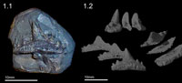
A single fossil shark tooth of Sphenacanthus hybodoides (Egerton, 1853) (accession number NHMUK PV P.1322) was utilized to demonstrate the potential benefits of micro-CT investigation. This freshwater shark species was found at Longton, Staffordshire, England (see Maisey, 1982; Dick, 1998) and lived during the Late Carboniferous approximately 315 MYA. Half of the fossil is embedded in matrix, and its digital preparation requires the full repertoire of extraction procedures (Figure 1.1). Yet the relatively simple structure of the tooth allows a virtual preparation to be carried out reasonably quickly, approximately 16-40 hours for a beginner or 4 hours for an expert (Figure 1.2). The original NHMUK (London) copyrighted micro-CT dataset of the fossil, comprising a tiff stack, are available from co-author Martha Richter for private (non-commercial) practice of the described techniques. In order to use the data to practice, one must first understand how CT data is collected and what it actually consists of.

HOW DOES A CT SCANNER WORK?

All micro-CT systems employ the same basic principles. Check the glossary for definition of terms. First the fossil is radiographed from many different directions to map density distribution, as measured by X-ray transmission. Then computer software is used to reconstruct the 2D radiographs into a 3D volume. During this step the data is usually processed to remove artefacts (mistakes) that invariably appear in CT scans, e.g., 'noise.'

Radiography

The Sphenacanthus tooth was scanned using an HMX-ST 225 CT System (Nikon Metrology, Tring, UK). The system consists of three key components: an X-ray source, a turntable and an X-ray detector panel (2000x2000 pixels). The X-ray source produces a cone-shaped X-ray beam by bombarding a metal target with electrons, generated by passing a high-energy electric current through a tungsten filament. The cone is focused onto a fossil, which is mounted on the turntable and rotated through 360º. During the rotation the detector panel collects a series of two-dimensional projections (radiographs) usually at between 0.1º to 0.05º intervals. The projections measure the amount of X-ray energy transmitted by the fossil. In order to produce a radiograph with high contrast and brightness, the X-ray beam must adequately penetrate the sample without over-exposing the panel. Hence the energy of the X-rays (determined by the voltage and current) has to be carefully selected by the CT user. Penetration of the beam (and projection contrast) is largely determined by the voltage, whilst the number of X-rays (and projection brightness) is mainly determined by the current. The fossil shark tooth was scanned with an X-ray beam set at 180 kV and 138 µA. A larger or denser fossil would require higher settings. It is worth noting that CT scans of dense specimens at high x-ray energy are likely to include beam-hardening artefacts, which can be reduced using filtration techniques.

Computer Reconstruction

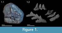
After scanning, a computer is used to line up and centre the projections in a radial pattern, rather like the spokes of a bicycle wheel. Each row of pixels in the detector panel will become a slice, so a cross-section of the specimen is created from each line of pixels in the radiograph using a method called back projection. Essentially, the projections for each slice are converted to digital profiles then smeared across each other to create digital images of the corresponding CT slices (see Figure 2). Each slice is made up of voxels, i.e., three-dimensional pixels. A CT reconstruction (or volume) is thus essentially a matrix (rather like a Rubik's cube). Each voxel is assigned a CT number or grey value. This value is based on the X-ray density (i.e., linear attenuation coefficient) of the materials being scanned (Zonneveld, 1987). The coefficient is a measure of the absorption (and scatter) of an X-ray beam as it passes through a material and is dependent largely on the density (but also thickness and atomic number). Thus a CT scan is akin to a 3D extension of a greyscale digital photograph, but based on X-ray transmission rather than visible light. The size of the voxels is determined by the magnification of the projected fossil image on the panel. The turntable can be moved to varying distances between the X-ray source and detector until the projection of the fossil fills the panel. The best magnification possible therefore is one where the voxel size is 1/2000^th of the width or height of the fossil (whichever is greater). Voxel size is a key concept in CT, because the dimensions (largely) determine the spatial resolution of the scan, i.e., the ability to resolve two objects of similar density that are situated close to one another. This value is usually between two and five times the size of the voxels. For the shark tooth, voxel size was 0.009 mm, and the effective spatial resolution was ? 0.050 mm.

Artefact Reduction

Micro-CT computer reconstruction is prone to artefacts (errors and mistakes). Artefacts are usually manifested as a blurring of material boundaries or a grainy appearance. The errors are caused by several aspects of CT such as the matrix (voxel) structure of the volumes, the properties of X-ray beams, X-ray scatter and electronic errors in the digital detector panel. The most commonly encountered artefacts, partial volume averaging effects and noise, greatly affect the spatial resolution. Volume averaging results from numerous linear attenuation coefficients (i.e., materials of different density) occupying a single voxel, and being represented by an averaged grey value. This phenomenon leads to a gradient of CT values at material interfaces (e.g., fossil and matrix) that appear to the naked eye as blurring of boundaries (Spoor et al., 1993; Zonneveld, 1987). The greater the size of the voxels relative to the width of anatomical features the greater the extent of the blurring. Fine features below the size of a voxel can become too blurred to visualise, or even disappear completely (but see McColl et al., 2006).

At very small voxel size, noise often becomes the factor limiting spatial resolution. All scans contain noise: unusually bright and dark voxels are superimposed over the CT data, which gives CT scans a grainy or speckled appearance, leading to blurring of material boundaries. X-ray scatter, which causes the photons to follow a non-linear path to the detector, can cause speckling, as can variation in the ability of pixels in the panel to detect X-rays. The extent of the speckling is determined by the signal (i.e., X-ray energy) to noise (i.e., error) ratio.

Another artefact commonly associated with dense objects like fossils is beam hardening, which is caused by variation in the energy of the X-ray beam. Micro-CT scanners produce polychromatic beams, i.e., X-rays of more than one wavelength. Hardening is the process of selective absorption of low energy X-rays from the polychromatic beam. As low energy X-rays are absorbed or scattered by a fossil, the beam becomes progressively harder or more penetrating. Thus the material at the edge of a fossil appears to be more dense (i.e., greater X-ray absorption) than the centre (i.e., lower X-ray absorption). The artefact is manifested in CT slices as a cupping of the CT numbers: a ring of excessively bright voxels around the edge of the fossil reducing to excessively dark voxels at the centre (see Ronan et al., 2010, figure 2). It is possible to reduce beam-hardening artefacts by scanning perpendicular to the long axis of the fossil (i.e., mount it standing up) or placing a copper filter in between the X-ray source and the fossil. The filter removes low energy X-rays and reduces the cupping artefact. By experimenting with different thicknesses and exposure times for the projections, it is usually possible to remove beam-hardening artefacts altogether. Alternatively, data processing algorithms can be used to remove the artefact post-scanning. To do this, it is possible to plot a transect across the centre of the specimen and calculate a second or third order polynomial that describes the variation (cupping) in grey values. The inverse of this polynomial can then be applied to even out the grey values. For a full discussion of beam-hardening artefacts and their removal see Ronan et al. (2010, 2011).

HOW AND WHERE DO I GET A CT SCAN?

The best option for obtaining a CT scan is to approach a centre of excellence, which carries out collaborative research with external users. Examples in the UK include: Imaging and Analysis Centre, Natural History Museum, London; Vis-µ, Southampton University; the School of Materials, University of Manchester; Department of Archaeology and Anthropology, University of Bristol; and CT @ SIMBIOS, University of Abertay. Collaborative scanning has many benefits because users can rely on experienced computed-tomographers to obtain high density-contrast scans, and then concentrate on the downstream data processing, which usually requires special anatomical knowledge. Furthermore, this type of contract scanning is actually very cheap. Charges vary but users can expect to pay between £10-120 per scan (see Abel et al., 2011). It is possible to include more than one specimen in a single scan, providing the voxel size will be small enough to image the anatomical features of interest. Alternatively, systems are becoming more affordable for scientists, so research groups can purchase their own as many Universities and Museums are choosing to do. A bench top SkyScan system or a cabinet Nikon Metrology system will cost about £150-250K.

HOW DO I PREPARE AND DISSECT A 'VIRTUAL' FOSSIL?

Since scans are becoming increasingly easy and cheap to obtain, a lack of training in imaging processing appears to be the major factor limiting CT based research. Software manuals are usually very technical and do not provide a workflow. This contribution hopes to bridge that knowledge gap by presenting a workflow that users can follow with an exemplar CT data set. Users have a wide variety of software packages, so this section contains a general description of the tools available to researchers. Specific advice on suitable software choices is provided later.

The example explored herein is a virtual preparation and dissection of the fossil shark tooth scan described above. The techniques suggested here can be applied for any CT scan of a specimen, either extinct or extant, by following a systematic workflow (Table 1). The tooth was partially embedded in rock matrix, and one of the objectives was to investigate the internal network of spaces originally occupied by vascular channels. Virtual preparation and dissection of the specimen - in this case, the whole fossil tooth and its internal vascular canal system - involved separating a scan into regions of interest (ROI). These corresponded to rock matrix, dental tissues like dentine and enameloid and, vascular canals (voids). The process of dividing the voxels in a 3D volume between discrete ROIs is termed segmentation. Regions were identified by common properties such as voxel grey value and/or location. Specifically, segmentation of the fossil was carried out in four steps using: contrast enhancement; surface determination; ROI growing and masking tools.

Density Contrast Enhancement

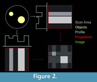
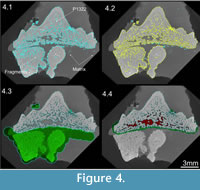
A contrast enhancement was applied to the whole stack of X-ray slices in order to better discriminate the grey values that represented fossil and matrix. A frequency distribution plot of voxel grey values (i.e., grey values vs. number of voxels) was stretched and compressed by altering the floating-point range. This numbering system registers grey values as decimals rather than integers in order to economise on the size and speed of the reconstruction (see Cline et al., 1998; Xu and Mueller, 2005). When the data is read into CT software the decimals are displayed as integers for ease of visualisation and manipulation by the end user. Reducing the upper end of the floating-point range (i.e., removing the brightest voxels) stretched the spread of mid-range grey values (e.g., fossil) at the cost of reducing the range of higher CT numbers (e.g., matrix). Producing a fequency distribution plot (Figure 3) and slice stack (Figure 4.1) with clearly distinguished matrix and fossil phases. This procedure greatly simplified and increased the speed of the rest of the segmentation process.

Surface Determination

The simplest and quickest way to segment an ROI is to separate the maxima (nodes) in the grey value frequency distribution plot (Figure 3) by applying a global threshold at the minima (valleys), which separate the nodes (See McColl et al., 2006; Reissis and Abel, 2012). Any voxels with a grey value above the threshold value are grouped in an ROI and those, which fall below, are discarded or made transparent. The frequency distribution graph for the fossil shark tooth reveals three peaks representing air, mineral-filled spaces and rock matrix as well as the fossil (Figure 3). The fossil ROI was defined by applying a global threshold at the grey value minima that separated the matrix peak from the fossil (Figure 3). The calibration was converted into an ROI (Figure 4.1 - cyan boundary). ROIs can be renamed in a meaningful way; in this case one ROI was created for the voxels representing any biologically mineralized tissues that make up the tooth (dentine and enameloid). However, since there were also fragments from other teeth embedded in the matrix, the tooth region of interest automatically included more than one fossil (Figure 4.1 - cyan boundary). This ambiguity can be resolved at a later stage (see below).

Region Growing

The fossil tooth was separated from other fragmentary remains by incorporating information regarding location. This separation was achieved using a 3D region-growing (or magic wand) tool. Region growing is an image processing technique that segments all voxels that are connected to a seed point and that are within a user defined tolerance(visually of same density) of voxel grey values (see Ronan et al., 2010). The larger the tolerance the more voxels will be selected. By searching only within the calibrated ROI it was possible to remove all non-adjacent teeth and fragments. Wand tools are most successful when the seed represents a low intensity voxel from the fossil (i.e., enameloid). By searching within the calibrated ROI (Figure 4.1 - cyan boundary) using a seed value of 45571 and a threshold of +20000 it was possible to create a new region of interest (Figure 4.2 - yellow boundary), which excluded some extraneous dental fragments (Figure 4.2 - cyan boundary). However, some adjacent unwanted material remained linked to the ROI.

Masking

Together, surface determination and region growing are not usually quite sufficient to completely prepare a fossil. Some regions of matrix or adjacent fragments must be manually removed using a process referred to as masking. This is typically the most time consuming, subjective and (usually) unavoidable aspect of segmentation. Voxels are manually added or removed from an ROI slice by slice (up to 2000 of them) or sets of few slices using a drawing or eraser tool (Figure 4.3 - green area). In our example the calibrated and region- grown ROI (Figure 4.2 - cyan boundary) was masked using an eraser tool (Figure 4.3 - green area) to produce a final, virtually prepared fossil, which could be dissected (Figure 4.4).

Virtual Dissection

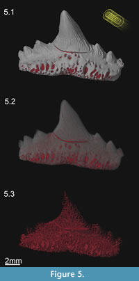An ROI representing the vascular system of the tooth was dissected using a combination of the region growing and masking tools. Voids representing the canals were extracted using the wand. The voids were continuous with the rock matrix though because of mineral infillings during the fossilization. Hence it was necessary to block (mask) the openings of the dental foramina. The foramina were blocked in 3D by manually creating small regions of interest slice by slice using a drawing tool (Figure 4.4 - green ROI). The wand tool was instructed to search within vascular canals in 3D from a starting seed point inside the void with a relatively pixel value of 32666, and the wand tolerance was set at +20000. The wand was instructed to 'avoid' other defined regions of interest, i.e., fossil tooth and blocking mask. Hence the tool only selected the vascular canals without spilling outside the fossil tooth (Figure 4.4 - red ROI). The creation of a region of interest produced a 3D segmentation of the vascular network, which could be visualised independently from the rest of the tooth (Figure 5).

In this case study, the virtual reconstruction reveals in great detail the external features of the tooth, as well as the internal dental anatomy (see Fischer et al., 2010), including most of the morphology of the vascular system (Radinsky, 1961), the type of dentine (trabecular versus ortho dentine) and the distribution of the enameloid cover on the crown (see Botella et al., 2009). Hence the virtual specimen reveals more information about the tooth than a mechanically prepared specimen would, even if it was sampled destructively by sectioning or chemical preparation, as the reconstruction and gross histological features are shown in 3D. However, the virtual dissection includes cracks in the tooth that are continuous with the vascular canals. Consequently there are some errors in the final prepared and dissected tooth (Figure 5). Given more time, these errors could be corrected. Users need to decide whether further segmentation is required given the scientific questions at hand or the desired quality of the virtual preparation.

HOW CAN I VISUALISE AND SHARE A VIRTUAL FOSSIL?

A CT scan is essentially a matrix made up of grey-scale voxels. The segmentation process simply groups the voxels together and defines them as materials/phases/tissues etc. The first segmentation and virtual preparation of fossils was relatively recent (Kearney et al., 2005; Balanoff and Rowe, 2007) but the technique is rapidly becoming a standard in palaeontology. In order to visualise a whole fossil or the segmented anatomical features the voxel data must be imaged or animated. In the same way that one might create photographic stills or videos of the original fossil. It is worth noting that the protocols discussed here can also be applied to process any voxel based datasets produced using 3D imaging modalities such as MRI, synchrotron tomography and confocal microscopy.

Volume Rendering

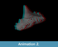
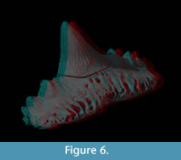Rendering is the process of generating an image from a 3D segmented volume using computer software. The segmented tooth and vascular system were rendered using lights, colour, stereo-perspective (Figure 5) and stereo-anaglyphy (Figure 6). Firstly the colour of the fossil was selected to resemble the original specimen, and the vascular system was reddened. Secondly, 3D perspective was applied to the virtual fossil by making the more distant parts of the object smaller than those close to the viewer, i.e., spatial shortening. Thirdly, creating shadows enhanced the sense of perspective. Two directional light sources were simulated; an ambient light directed straight at the specimen and a spotlight angled from the upper left, as is customary in photography (Figure 5.1). The exact position of the lights was adapted to match each rendering of the tooth/vascular system and set the surface markings or vascular system in clear contrast (Figure 5.2-3). The manner in which light reflected off the 'virtual' fossil tooth was modelled using the Phong algorithm (Phong, 1975) where rough and smooth surfaces reflected light in specular and diffuse patterns respectively. Finally, a stereo-anaglyph was created to provide a full stereoscopic 3D effect, when viewed with red-cyan spectacles (Figure 6, Supplementary File 2).

Movie Animation

Animation is an excellent tool for sharing datasets and can be used to draw the eye of the end viewer to specific features of interest. Movies also allow a degree of interactivity with the user able to visualise a fossil from different angles and perhaps make independent interpretations about the morphology (see Parfitt et al., 2010, Abel et al., 2011). In order to demonstrate the quality and usefulness of the virtual fossil, an animation, rotating once about the long axis, was created (see Supplementary File 1). The simple animation depicts a camera flying around the tooth whilst the fossil becomes transparent to reveal the vascular canal system inside (see Supplementary Files 1, 2). 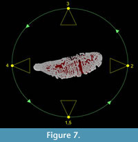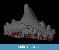This effect was achieved using key framing: a technique based on traditional hand-drawn animation. Senior animators would draw the key frames from an animation sequence then a junior assistant would draw the frames in between. Computerised key framer applications work in a similar way by interpolating an animation across user-defined key frames or camera views. In this case, five evenly spaced key frames were defined around the specimen, each frame was 45º apart, except the first and last frames, which were both located at 0º (Figure 7). Thus the movie starts and ends at the same position. At each key frame the rendering settings were defined, e.g., camera angle, lighting and tooth transparency. The key framer then automatically interpolated the complete path of the camera and rendering settings to create the 360º fly around. The videos are small enough to email (<16Mb) and can be embedded in PDF files or added to publications as downloadable supplementary information.

Stereolithographic Files

It is possible to create even smaller files by converting CT datasets to stereo-lithographic (STL) files. An STL file is a surface mesh (usually triangles), which describes both the internal and external geometry of a three-dimensional object. Creation of an STL file is akin to physically stretching a triangular mesh over the voxels in the virtual model creating a smooth appearance of the voxels and slicing them into a continuous surface. Example STL files of the tooth (Supplementary File 3) and vascular system (Supplementary File 4) were built. The files can be opened up in many 3D imaging software packages (see Table 2). Users can manipulate, rotate and section STL files. Hence they are less restricted and more interactive than animated movies, but end users require better computer software skills.

WHICH SOFTWARE SHOULD I USE TO CREATE 'VIRTUAL' FOSSILS?

A huge number of commercial and freeware packages are available for segmentation and rendering CT data. The most widely used packages are listed in Table 2 along with a synopsis of functionality and a list of URLs. The ability of the programmes to accomplish the key CT data processing steps varies. The data processing steps incorporated within each programme are highlighted in Table 2. Ultimately each CT user must select appropriate software based on the particular data processing tasks required.

We have found that generally the most useful software packages for processing scans of fossil are VGStudio MAX 2.1 (Volume Graphics, Heidelberg, Germany) SPIERS (Selden et al., 2008; Garwood et al., 2009) and Drishti (Jones et al., 2007; Sakellarioua, 2007). For this paper the shark tooth CT data was post segmented and rendered using VGStudio MAX 2.1 because the programme includes all of the data processing tools discussed here. Since the programme can carry out thresholding and segmentations in 3D using surface determination and wand tools the speed at which fossils can be segmented is faster in comparison to most other software packages. However, the base package costs around £9K, but is available for less with academic discounts. SPIERS is a simple but highly capable programme for slice based (i.e., 2D) masking segmentation of CT data making the programme ideally suited to many fossils, particularly those with low density contrast scans. In contrast, Drishti is not as useful for thresholding or segmenting CT data and is rather restricted to basic image contrast enhancement. However, the programme is excellent for rendering movie animations, spins or flythrough, of fossil specimens. Alternatively excellent movies can be produced using open source software such as SPIERS to create STL files then animating them using, e.g., BLENDER. Ultimately advising users which software packages to adopt is not straightforward. Users' requirements are often esoteric but SPIERS is a useful (free) place to start and is well supported by the authors (Garwood et al., 2009; Garwood et al., 2010; Garwood and Sutton, 2012; Sutton et al., 2012).

HOW DO I MEASURE A 'VIRTUAL' SPECIMEN?

Sphenacanthus was originally CT-scanned because of the scientific interest in describing its internal dental anatomy and gross histology, such as the type of dentine that makes up the crown and base of the tooth. The voxel based micro-CT scan is a mathematical representation of an object, rather than an image, which contains accurate scale information and is therefore suited to the quantitative analysis of geometry and structure in 3D. For example, dental crown morphology has been characterised using landmark-based geometric morphometric measures collected directly from CT scans (Gomez-Robles, 2007, 2008). There are many programmes for collecting landmark data such as Stratovan Checkpoint (see Table 2). Similarly the structure of the vascular network could be measured using ImageJ (Abramoff, 2004) plugins such as BoneJ (Doube et al., 2010). Originally intended for analysing bone, the software can calculate the thickness, connectivity and orientation of trabeculae (cancellous bone). However, the software could be co-opted for measuring vascular structure. For a description of how the measures are calculated visit BoneJ.Org.

However, it is important to note that the accuracy of measurements collected from CT Scans will be affected by the quality of the scanning and segmentation. Scanning artefacts such as partial volume averaging, noise and beam hardening obscure material boundaries within a CT scan. Hence, segmentations based on surface determination, region growing or masking will not be entirely accurate. Furthermore, segmentation is a subjective process. Selection of global thresholds, wand seed points and tolerance varies across users. Similarly manual masking is a subjective process, which relies heavily on the prior anatomical knowledge of the user. Therefore, users should assume that segmentations are subject to error and (where possible) avoid measuring features close to or smaller than the resolution of the scan. As a rule of thumb this would be no smaller than two to five times the voxel size. Scan resolution can be determined accurately by scanning and measuring plastic (TEM) grids with meshes of varying size. The grids can be scanned alongside a fossil or separately, the finest grid that can be visualised and measured is equal to the resolution of the scan.

HOW CAN I DISSEMINATE VIRTUAL COLLECTIONS?

Quantitative analysis of fossil geometry can require large comparative samples. Museums and universities are starting to build up and share significant 'virtual collections' of specimens. The first attempt to systematically distribute fossil CT data was made by Rowe and colleagues (Rowe et al., 1993, 1995). The reptile fossil Thrinaxodon was scanned and slice stacks made available on CD. This was a landmark in CT and more generally in the Natural Sciences. Since then the Internet has allowed researchers to share data more directly, for example via the inspeCT applet on DigiMorph. Other organisations such as NESPOS and the Natural History Museums (London, UK) are also sharing CT data. However, the advancement of CT based morphological research is being held back by a lack of significant data archives available for download and visualisation at full resolution (see Rowe and Frank, 2012), even though the technology and software for sharing data sets across the Internet is already available to most users.

Segmented or un-segmented datasets can be easily disseminated across the Internet in a few hours with the use of ftp sites. Provided that a Secure File Transfer Protocol (SFTP) encryption is used, the data can be transported safely (Abel et al., 2011). The file size of CT datasets may be the factor limiting storing and dissemination of CT datasets. A set of projections from a CT scan can be 25 GB in size, and the reconstructed 3D volume can be 32 GB. Consequently data sets are often downsized from 32/16-bit to 8-bit, and although the compression reduces contrast density this is usually sufficient for most users' needs. Particularly when there are only three phases, e.g., air, matrix and fossil. Alternatively, data can be stored as JPEG2000 format, which has a very high compression with minor loss of information. However, creating and uncompressing 32 GB of JPEG 2000 files can take 30 minutes or more.

STL files can be emailed or file exchanged very quickly or added as supplementary information to a paper. Typically STLs are only a few tens or hundreds of megabytes in size. An STL file can also be rapidly prototyped to produce a 3D plastic model (see Abel et al., 2011). Models are built using 3D printers by tracing out a stack of CT cross-sections in layers of UV-curable resin. This mirrors the creation of a CT volume from a slice stack to a great extent. The resolution of the models is usually between 0.5 to 0.1 mm, which is usually high enough to capture fine surface topology. The resin models can be scaled up or down for use in education and research, e.g., in museum galleries, schools and universities. When conceptualising the size and shape of fossils, many users, particularly students and school children, may find that 3D prints are more useful than virtual models.

DISCLAIMER: IS MICRO-CT A 'SILVER BULLET'?

The majority of fossils cannot be scanned using current CT technology. Palaeobiologists must carefully consider whether a given fossil is suitable for CT, or whether a more traditional technique would be more useful. There are various reasons why fossils cannot be scanned. Firstly, much of the paleontological record (estimated at ~90%) consists of specimens flattened by the fossilisation process. Flat objects are usually very difficult to CT scan because of the unequal path length for x-rays. The broadside is often overexposed while the edges are underexposed.

Secondly, for 3D fossils, size and density are the main limiting factors. A scanner must be large enough to accommodate a specimen and powerful enough to produce X-rays that can penetrate the material. Most commercially available scanners do not have a field of view greater than 250 mm in diameter and height (e.g., HMX-ST CT System, Nikon Metrology, Tring, UK). Furthermore, most systems can only generate X-rays with energy of between 20-450 kV. At maximum power a 225 kV system can penetrate a block of limestone 100-200 mm in diameter whilst a 450 kV system can penetrate a lump of ironstone, which is 50-100 mm across.

Thirdly, in order for the scanner to distinguish the materials in a scanned fossil, e.g., bone and matrix, there must be sufficient density contrast between them. Where two materials have similar densities, the voxels that represent the tissue will have comparable grey values to the host rock. If this is the case, blurring caused by partial volume averaging effects is compounded, and noise prevents segmenting. For equivalent voxel size at low-density contrast, such as a calcite fossil in limestone, the blurring is greater than at high-density contrast such as a fossil void in siderite. Enhancement can improve grey value contrast between two materials, but tends only to be useful when there is already reasonable contrast, and the user wants to create a sharper cutoff for masking (manual) segmentation (Dominguez et al., 2002).

It is also worth mentioning that CT is not a substitute for other techniques aimed at resolving morphological features of biological materials at fine histological level. An example is light microscopy of thin-sectioned specimens. Although actual (as opposed to virtual) thin-sectioning is a 'destructive' sampling technique, it can be justified and necessary in a number of cases, for instance when CT cannot resolve structures such as cell spaces, dentinal tubules or Sharpey fibers. Although some CT systems are capable of resolving features at the nano-scale (e.g., nano-CT, Synchrotron and XuM).

CONCLUSONS: WHAT NEXT FOR CT?

Micro-CT is a powerful non-destructive imaging modality for the full-volume visualization of both the external and internal aspects of an object in 3D. Hence it has become very popular in biological research, allowing the rich detail of internal structures to be retrieved, without any damage to the specimens (see Elliot and Dover, 1982; Flannery et al., 1987; Rowe et al., 1997). However, as seen above, computed tomography is not a suitable technique for all fossils. Scanning is limited by the overall size and density of a fossil as well as the density contrast between phases, e.g., matrix and bone, and relies on three-dimensional preservation. Where applicable virtual preparation does have several advantages over mechanical preparation. Digital preparation is quicker than many mechanical or chemical preparations. The digital process requires less training and experience, approximately 1-2 days of training. Few research institutions and museums can afford to employ fossil preparers, who develop their highly specialized professional skills through many years of experience.

Furthermore, the original fossil and host matrix context is not destroyed or damaged in any way through CT scanning. Since fossils are not always completely visible at the start of the preparation process, it is possible to make mistakes that can damage the specimen. Every mechanical or acid preparation of fossils is therefore a unique exercise that is also usually very time consuming and costly. The original CT data can be curated along with actual specimens, providing a permanent digital record of the specimen. Should practices change or imaging processing software improve, then virtual preparations can be repeated utilising the original scan. Presently the CT technique is still waiting for further innovations that will bring the technology into mainstream research. This technology would be attributable to three factors, affordability, productivity and computing power.

Firstly, systems and scans are becoming more affordable for museums and universities so at some point every institution will have CT and computer laboratories as standard. Secondly, scan time and field of view, which limit the number and size range of specimens that can be scanned, are constantly improving. Some systems such as the HMXST CT (Nikon Metrology, Tring, UK) can already collect a scan in 10-20 minutes. New systems are being developed incorporating automatic scanning and specimen changes. Allowing systems to run over weekends and holidays will also greatly increase CT capacity. The field of view is also increasing. The size of detector panels doubles every two years, and new software algorithms allow scans to be stitched together. Using the HMX-ST system, which has a field of view 250x250 mm, it is possible to scan an object 1000x250 mm in four sections and stitch them together virtually. At the present some manual labour and patience on the part of the user is required but sooner or later this function will be automated. Hence, museums and universities will be able to build up significant 'virtual collections' from a varied array of specimens and materials. Thirdly, computing power is increasing dramatically relative to cost. Until recently, computing power lagged way behind CT scanning technology. It is only in the last five years that computer prices have fallen enough for an increasing number of palaeobiologists to invest. At present a PC suitable for segmenting and rendering will require about 2TB of storage and 64 GB of RAM but costs only £5K. However, in order for collaborators to share large datasets on powerful computers we will need faster Internet speeds.

Despite these ongoing and future developments, we still have a long way to go in order to make entire museum or university collections available to scientists and the public alike in digital form. The Natural History Museum in London alone contains approximately 75 million specimens, which amounts to generations worth of scanning, reconstruction, preparation, dissection, rendering, measurement and quantitative analysis. However, if we could routinely exploit CT and other 3D imaging techniques to share data more widely either freely or at a low cost, we could be ushering in a new era of global scientific collaboration and public communication. CT scanning is an unbeatable technique for discovering hidden fossils inside rocks and internal features of specimens that until now have been impossible to visualise without destroying them.

ACKNOWLEDGMENTS

The authors would like to thank: R. Garwood (The University of Manchester); T. Rowe (The University of Texas at Austin); A. Ramsey (Nikon Metrology, Tring, UK) and D. Handl (Volume Graphics, Heidelberg Germany) for helpful comments and advice as well as A. Ball and L. Howard (Natural History Museum, London).

REFERENCES

Abel, R.L., Parfitt, S.A., Ashton, N.M., Lewis, S.G., and Stringer, C.B. 2011. Digital preservation and dissemination of ancient lithic technology with modern micro-CT. Computers and Graphics, 35:878–884.

Abramoff, M.D., Magelhaes, P.J., and Ram, S.J. 2004. Image processing with ImageJ. Biophotonics International, 11:36-42.

Balanoff, A.M. and Rowe, T.B. 2007. Osteological description of an embryonic skeleton of the extinct Elephant bird, Aepyornis (Palaeognathae, Ratitae). Memoir 9, Society of Vertebrate Paleontology, Journal of Vertebrate Paleontology, Supplement to 27:1-54, plus supplementary CD-ROM.

Botella, H., Donoghue, P.C.J., and Martinez-Perez, C. 2009. Enameloid microstructure in the oldest known chondrichthyan teeth. Acta Zoologica, 90:103-108.

Cline, H.E., Lorensen, W.E., Ludke, S., Crawford, C.R., and Teeter, B.C. 1998. Two algorithms for the three dimensional construction of tomograms. Medical Physics, 15:320-327.

Croft, W.N. 1950. A parallel grinding instrument for the investigation of fossils by serial sections. Journal of Paleontology, 24:693-698.

Dick, J.R.F. 1998. Sphenacanthus, a Palaeozoic freshwater shark. Zoological Journal of the Linnean Society, 122:9-25.

Dominguez, P., Jacobson, A.G., and Jefferies, R.P.S. 2002. Paired gill slits in a fossil with a calcite skeleton. Nature 417, 841-844.

Doube, M., K?osowski, M.M., Arganda-Carreras, I., Cordelières, F., Dougherty, R.P., Jackson, J., Schmid, B., Hutchinson, J.R., and Shefelbine, S.J. 2010. BoneJ: free and extensible bone image analysis in ImageJ. Bone 47:1076-9.

Egerton, P.M.G. 1853. Palichthyologic Notes No 5 - On two new species of placoid fishes from the Coal Measures. Quarterly Journal of the Geological Society of London, 9:280-282.

Elliott, J.C. and Dover, S.D. 1982. X-ray microtomography. Journal of Microscopy, 126:211-213.

Fischer, J., Schneider, J.W., and Ronchi, A. 2010. New hybodontoid shark from the Permocarboniferous (Gzhelian-Asselian) of Guardia Pisano (Sardinia, Italy). Acta Palaeontologica Polonica, 55:241-264.

Flannery, B.P., Deckman, H.W., Roberge, W.G., and D'Amico, K.L. 1987. Three-dimensional X-ray microtomography. Science, 237:1439-1444.

Garwood, Russell J. and Sutton, Mark D., 2012. The enigmatic arthropod Camptophyllia. Palaeontologia Electronica Vol. 15, Issue 2;15A,12p;
palaeo-electronica.org/content/2012-issue-2-articles/218-the-arthropod-camptophyllia

Garwood, R.J., Dunlop, J.A., and Sutton, M.D. 2009. High-fidelity X-ray micro tomography reconstruction of siderite-hosted Carboniferous arachnids. Biology Letters, 5:841-844.

Garwood, R.J., Rahman, I.A., and Sutton, M.D. 2010. From clergymen to computers – the advent of virtual palaeontology. Geology Today, 26:96-100.

Gomez-Robles, A., Martinon-Torres, M., Bermudez de Castro, J.M., Prado, S., Sarmiento, S., and Arsuaga, J.L. 2008. Geometric morphometric analysis of the crown morphology of the lower first premolar of hominins, with special attention to Pleistocene Homo. Journal of Human Evolution, 55:627-638.

Gomez-Robles, A., Martinon-Torres, M., Bermudez de Margvelashvili, A., Bastir, M., Arsuaga, J.L., Perez-Perez, A., and Martinez, L.M. 2007. A geometric morphometric analysis of hominin upper first molar shape. Journal of Human Evolution, 53:272-285.

Hounsfield, G.N. 1973. Computerized transverse axial scanning (tomography): part I. Description of system. British Journal of Radiology, 46:1016-22.

Jones, A.C., Arns, C.H., Sheppard, A.P., Hutmacher, D.W., Milthorpe, B.K., and Knackstedt, M.I. 2007. Assessment of bone in growth into porous biomaterials using Micro-CT. Biomaterials, 28:2491-2504.

Kearney, M., Maisano, J.A., and Rowe, T. 2005. Cranial anatomy of the extinct worm-lizard Rhineura hatcherii (Squamata, Amphisbaenia) based on High-Resolution X-ray Computed Tomography. Journal of Morphology, 264:1-33, plus Web supplement at www.DigiMorph.org.

Maisey, J. 1982. Studies on the Paleozoic selachian genus Ctenacanthus Agassiz: No. 2. Bythiacanthus St. John and Worthen, Amelacanthus, new genus, Euemacanthus St. John and Worthen, Sphenacanthus Agassiz, and Wodnika Münster. American Museum Novitates, 2722:1-24.

McColl, D.J., Abel, R.L., Spears, I.R., Macho, G.A. 2006. Automated method to measure trabecular thickness from microcomputed tomographic scans and its application. Anatomical Record. Part A, Discoveries in Molecular, Cellular and Evolutionary Biology, 288:982-988.

McCormack, A.M. 1963. Representation of a function by its line integrals, with some radiological applications. Journal of Applied Physics, 34:2722-2727.

Parfitt, S.A., Ashton, N.M., Lewis, S.G., Abel R.L., Coope, G.R., Field, M.H., Gale, R., Hoare, P.G., Larkin, N.R., Lewis, M.D., Karloukovski, V., Maher, B.A., Peglar, S.M., Preece, R.C., Whittaker, J.E., and Stringer, C.B. 2010. Early Pleistocene human occupation at the edge of the boreal zone in northwest Europe. Nature, 466:229-233.

Phong, B.T. 1975. Illumination for computer generated pictures. Communication of the ACM, 6:311-317.

Radinsky, L. 1961. Tooth histology as a taxonomic criterium for cartilaginous fishes. Journal of Morphology, 109:73-92.

Reissis, D., and Abel, R.L., 2012. Development of fetal trabecular micro-architecture in the humerus and femur. Journal of Anatomy, 220:496-503.

Ronan, R., Abel, R.L., Johnson, K., and Perry, C. 2010. Quantification of porosity in Acropora pulchra (Brook 1891) using X-ray micro-computed tomography techniques. Journal of Experimental Marine Biology and Ecology, 396:1-9.

Ronan, R,. Abel, R.L., Johnson, K., and Perry, C. 2011. Spatial variation in porosity and skeletal element characteristics in apical tips of the branching coral Acropora pulchra (Brook, 1891). Coral Reefs, 30:195-201.

Rowe, T. and Frank, L.R. 2012. The disappearing third dimension. Science, 331:712-714.

Rowe, T., Carlson, W., and Bottdorf, W. 1993. Thrinaxodon Digital Atlas of the Skull, CD-ROM. University of Texas Press, Austin, 623 megabytes.

Rowe, T., Carlson, W., and Bottorff, W. 1995. Thrinaxodon: Digital Atlas of the Skull. CD-ROM (Second Edition). University of Texas Press, 547 megabytes.

Rowe, T., Kappelman, J., Carlson, W.D., Ketcham ,R.A., and Denison, C. 1997. High-resolution computed tomography: a breakthrough technology for earth scientists. Geotimes, 42:23-27.

Sakellarioua, A., Arnsa, C.H., Shepparda, A.P., Soka, R.M., Averdunka, H., Limaye, A., Jones, A.C., Senden, T.J., and Knackstedt, M.A. 2007. Developing a virtual materials laboratory. Materials Today, 10:44-51.

Selden, P.A., Shear, W.A., and Sutton, M.D. 2008. Fossil evidence for the origin of spider spinnerets, and a proposed arachnid order. Proceedings of National Academy of Sciences USA, 105:20781-20785.

Sollas, W.J. 1904. A method for the investigation of fossils by serial sections. Philosophical Transactions of the Royal Society of London. Series B, Biological Sciences, 196: 259-265.

Spoor, C.F., Zonneveld, F.W., and Macho, G.A. 1993. Linear measurements of cortical bone and dental enamel by computed tomography: applications and problems. American Journal of Physical Anthropology, 91:469-484.

Sutton, Mark D., Garwood, Russell J., Siveter, David J., and Siveter, Derek J. 2012. SPIERS and VAXML; A software toolkit for tomographic visualisation and a format for virtual specimen interchange. Palaeontologia Electronica Vol. 15, Issue 2;5T,14p; 
palaeo-electronica.org/content/94-issue-2-2012-technical-articles/226-ct-toolkits

Xu, F. and Mueller, K. 2005. Accelerating popular tomographic reconstruction algorithms on commodity PC graphics hardware. IEEE Transactions on Nuclear Science, 52:654-663.

Zonneveld, F.W. 1987. Computed tomography of the temporal bone and orbit. Munich, Urban and Schwarzenberg.