


FIGURE 1. Cephalon of Cryptolithus tesselatus (AMNH FI-101479) showing morphological terms used in this paper, following Whittington (1968) and Hughes et al. (1975). Concentric arcs are labeled according to their placement relative to the girder (expressed on the ventral side): E = external; I = internal. “Fringe-pits” are circled in yellow; the “F-pits” represent a subset of these interior to the labeled concentric arcs. Specimen is 6.6 mm long.
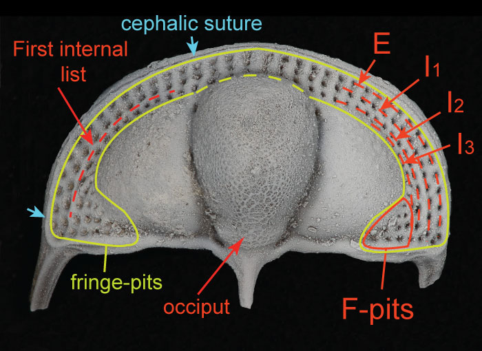
FIGURE 2. Different views of 3D surface model rendering of Cryptolithus tesselatus showing placement of fixed landmarks. All landmarks are indicated at least once, with the exception of 11 (paired with 12). Unpaired landmarks = 17-20; paired landmarks = 1-16, 21-23, 42; semi-landmarks along first internal list shown by dashed line and represented by landmarks 24-41. See Appendix 2 for full description of all landmarks. Surface reconstruction is of AMNH FI-101479.
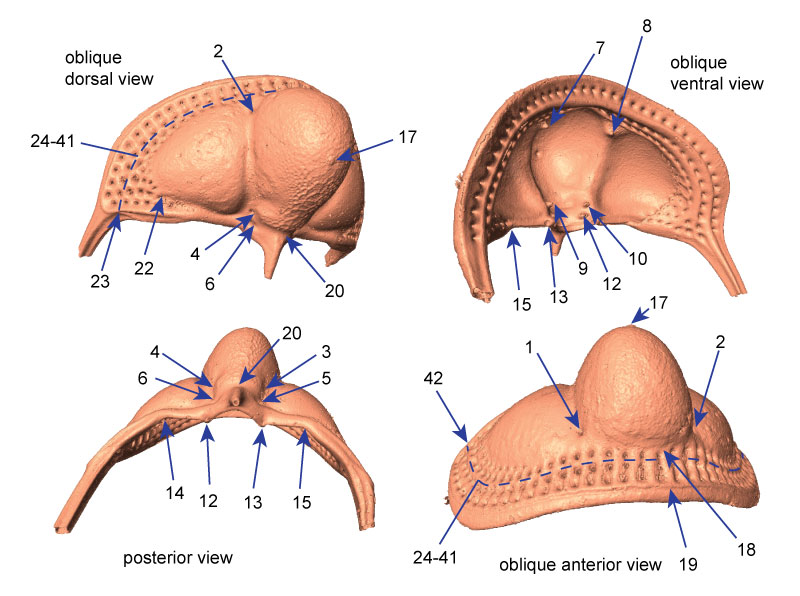
FIGURE 3. Placement of points defining patch on glabella. Points in red are redundant to fixed landmarks as described in the text and Appendix 2. After the surface landmarks were extracted using Landmark Editor, the redundant landmarks were removed from the final data file. Specimen shown is AMNH FI-101482; specimen is 7.1 mm long.
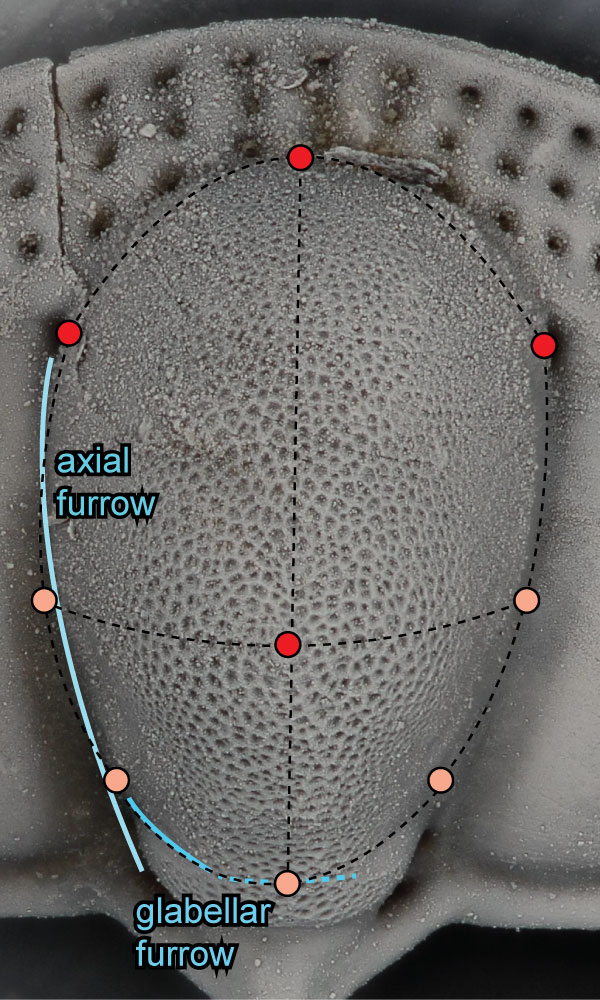
FIGURE 4. Slice through volume rendering of Cryptolithus tesselatus (AMNH FI-101479), shown in dorsal view in inset. Red line in inset shows the orientation of the slice across the specimen. Bright white area is sediment trapped within the bilaminar structure of the cephalon. Blue arrows point to suture between upper and lower lamellae; red arrows point to fringe-pits.
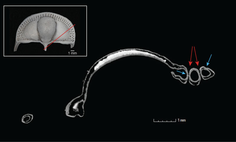
FIGURE 5. Principal components analysis of 3D fixed and semi landmarks. 1, PC 1 vs PC 2; point size represents relative centroid size of specimen. 2-4, Landmark configuration of shape represented by low PC 1 score, typical of largest specimens, in dorsal, anterior, and right lateral views, respectively. 5-7, Landmark configuration of shape represented by high PC 1 score, typical of smallest specimens, in dorsal, anterior, and right lateral views, respectively.
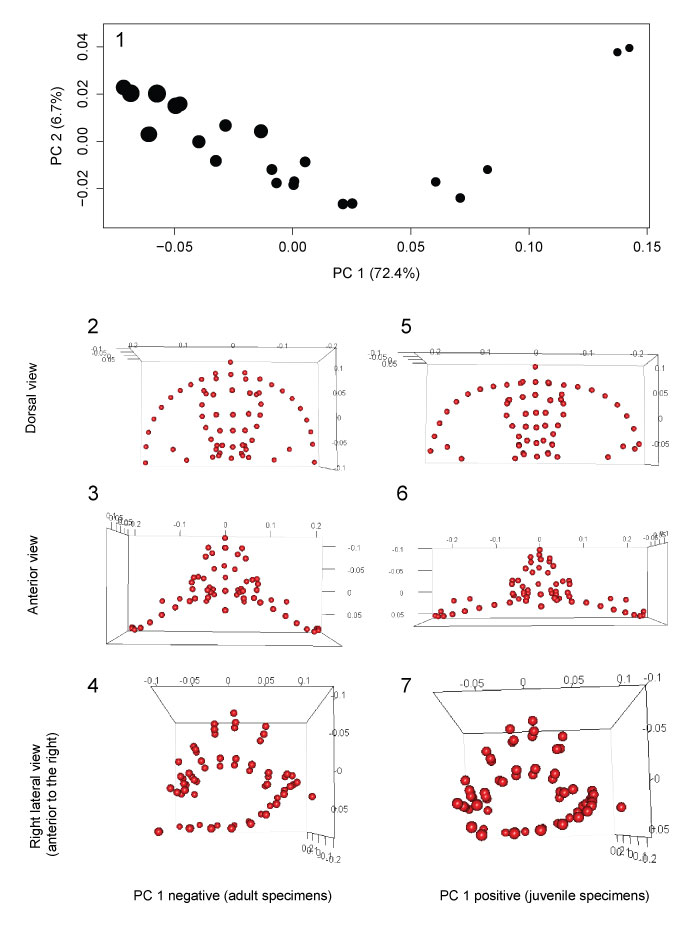
FIGURE 6. Allometric growth in Cryptolithus tesselatus. Size (x-axis) is represented by the natural log of centroid size. Change in shape (y-axis) is represented by the Procrustes distance between each specimen and the smallest specimen in the dataset; the Procrustes distances in this case represent the relative amount of change that specimens underwent during development. Red solid line = linear regression model; blue solid line = threshold model 1; thin black dashed line = threshold model 2; thick black dashed line = threshold model 3. Threshold model 1 is the best supported model.
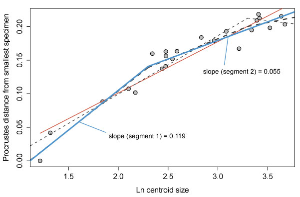
FIGURE 7. Additions of fringe-pits associated with early meraspid stages of ontogeny in Cryptolithus tesselatus. 1, meraspid stage 2 showing two concentric arcs of fringe-pits, AMNH FI-101498, x35. 2, meraspid stage 2 showing two concentric arcs of fringe-pits, AMNH FI-101499, x35. 3, merapid stage 3 showing three concentric arcs of fringe-pits and first few fringe-pits of I3, FI-101496, x20. 4, later meraspid stage showing complete set of fringe-pits, AMNH FI-101494, x15. Scale bars are 1 mm.
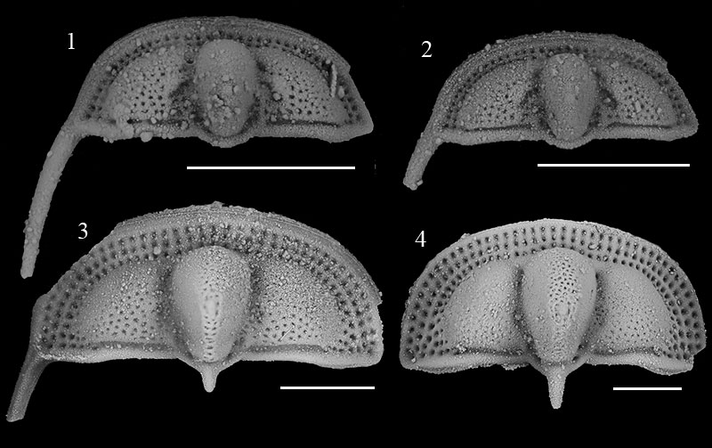
FIGURE 8. Length vs width of Cryptolithus tesselatus cephala, coded for the number of concentric arcs of fringe-pits expressed in each specimen. The first three concentric arcs (E, I1, and I2) are complete when first expressed. Based on clustering, I3 is likely completed over three molts, first by only 1-3 fringe-pits, then 8-10 fringe-pits, then 13-15 fringe-pits with the anteriormost in line with the 10th radial rows of fringe-pits in arcs E-I2. The dataset includes the 23 specimens, which were CT-scanned as well as 31 additional silicified specimens from the collection; specimens that were CT-scanned are outlined in red. Arrows indicate the specimens shown in Figure 1 and Figure 7. Inset in upper right corner is a magnified view of the specimens in the dashed box. The scaling component describing the relationship between length and width is 1.153 (1 = isometric growth).
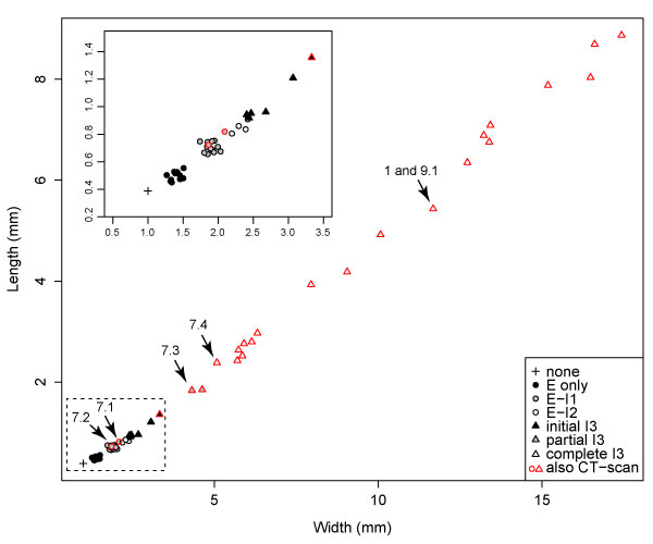
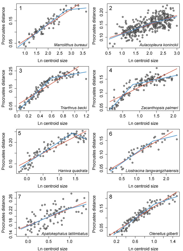
FIGURE 9. Ontogeny of Cryptolithus tesselatus based on 2D geometric morphometrics. 1, Fixed landmarks consistently recognizable in dorsal view. Red dashed line shows curve described by first internal list along which were placed 21 semi-landmarks. Specimen shown is AMNH FI-101479; specimen is 6.7 mm long. 2, Principal components analysis of 2D fixed- and semi-landmarks. Point size represents relative centroid size of specimen. Insets are deformation plots showing shapes represented by largest and smallest PC 1 values. 3, Allometric curve; amount of shape change represented by the Procrustes distance between each specimen and the smallest specimen. Red solid line = linear regression model; blue solid line = threshold model 1; thin black dashed line = threshold model 2; thick black dashed line = threshold model 3. Threshold model 1 is the best supported model (Table 1).
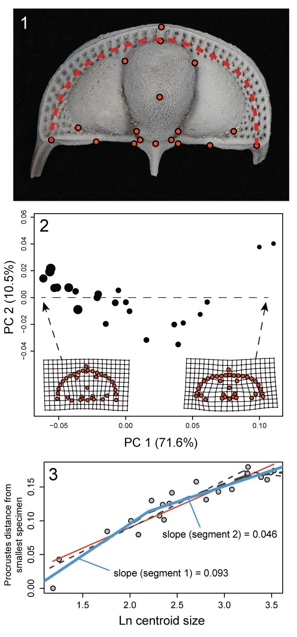
FIGURE 10. Allometry in the cranidia/cephala of other trilobite species as described by 2D geometric morphometrics. 1, Marrolithus bureaui, data from figure 5 of Delabroye and Crônier (2008), breakpoint shown is at 2.8, which was the best supported threshold model (Table 2). 2, Aulacopleura koninckii, data from figure 3 of Hong et al. (2014), breakpoint set at 2.0. 3, Triarthrus becki, data from figure 6 of Kim et al. (2002); breakpoint at 0.6. 4, Zacanthopsis palmeri, data from figure 13 of Hopkins and Webster (2009), breakpoint set at 0.8. 5, Haniwa quadrata, data from figure 5 of Park and Choi (2011b), breakpoint set at 1.4. 6, Liostracina tangwangzhaiensis, data from figure 3 of Park et al. (2014), breakpoint set at 1.55. 7, Apatokephalus latilimbatus, data from figure 4 of Park and Kihm (2015), breakpoint set at 0.85. 8, Olenellus gilberti, data from figure 23B of Webster (2015), breakpoint set at 1.0. Breakpoints are all in units of natural log of centroid size. Red lines = linear regression models; blue lines = threshold models.

 A Review of Handbook of Paleoichthyology Volume 8a: Actinopterygii I, Palaeoniscimorpha, Stem Neopterygii, Chondrostei
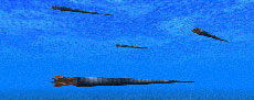 Palaeontologia Electronica among the most influential palaeontological journals