

Article Search
Volume 27.2
May–August 2024
Full table of contents
ISSN: 1094-8074, web version;
1935-3952, print version
Recent Research Articles
See all articles in 27.2 May-August 2024
See all articles in 27.1 January-April 2024
See all articles in 26.3 September-December 2023
FIGURE 1. The localities included in this study from England and Ireland (1.1) and from Germany (1.2). The maps (1.1) and (1.2) are not to the same scale.
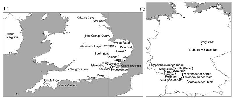
FIGURE 2. Linear regressions of mean mesowear values of the ungulates in the local palaeocommunities and NAP % in the pollen records of the localities with (1.1.) minimum NAP %, (1.2.) maximum NAP % and (1.3.) mean NAP %.
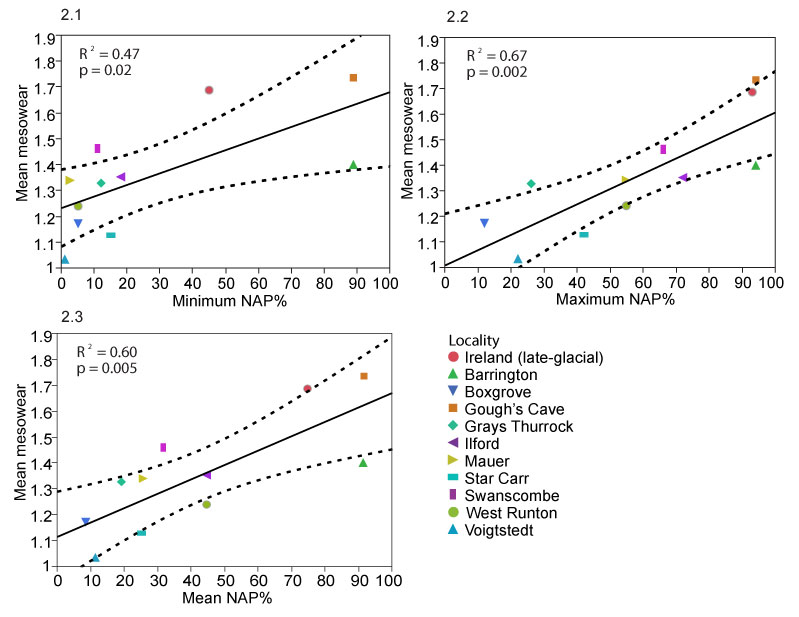
FIGURE 3. Linear regressions of mean mesowear values of deer (Cervidae) from localities with pollen records, and minimum, maximum and mean NAP % in the pollen records of the localities. Numbers of specimens per locality are given in brackets after the locality names. For Megacerini, the samples from Grays Thurrock and Ireland are Megaloceros giganteus ; those from Boxgrove, West Runton and Voigstedt combine Praemegaceros verticornis, P. dawkinsi and Megaloceros savini. For Dama the specimens from Boxgrove are D. cf. roberti ; others are D. dama.
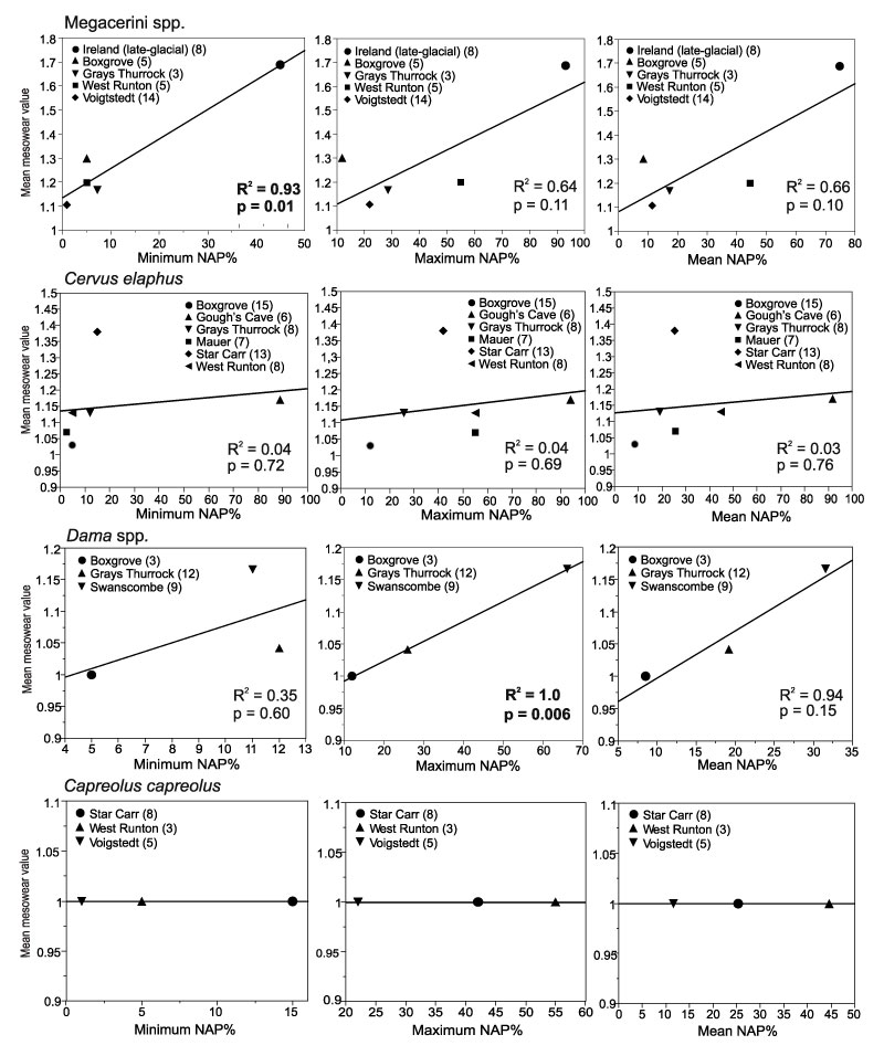
FIGURE 4. Linear regressions of mean mesowear values of Bovidae, Equus ferus and Rhinocerotidae from localities with pollen records, and minimum, maximum and mean NAP % in the pollen records of the localities. Numbers of specimens per locality are given in brackets after the locality names. Bison from Mauer is B. schoetensacki ; from other localities, B. priscus.
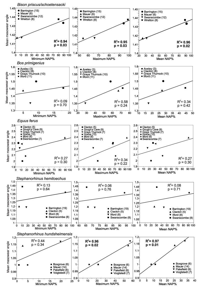
FIGURE 5. Linear regressions of body mass (kg) of deer (Cervidae) from localities with pollen records, and minimum, maximum and mean NAP % in the pollen records of the localities. Each point represents an individual specimen. Numbers of specimens per locality are given in brackets after the locality names.
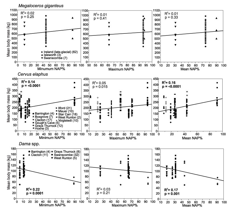
FIGURE 6. Body mass of Cervus elaphus, Dama spp. and Capreolus capreolus in Middle and Late Pleistocene localities from Britain and Germany. The localities are arranged from oldest (right) to youngest (left) estimated age. The middle line in the diamonds marks the mean body mass and the upper and lower lines mark the 95% confidence limits of the mean. Diamonds that do not overlap at the 95% lines indicate statistically significant difference between populations. The central line in the figures indicates the combined mean body mass of all the populations. The individual body mass estimates of each specimen are shown as data points. Sample sizes are given in brackets for each locality.
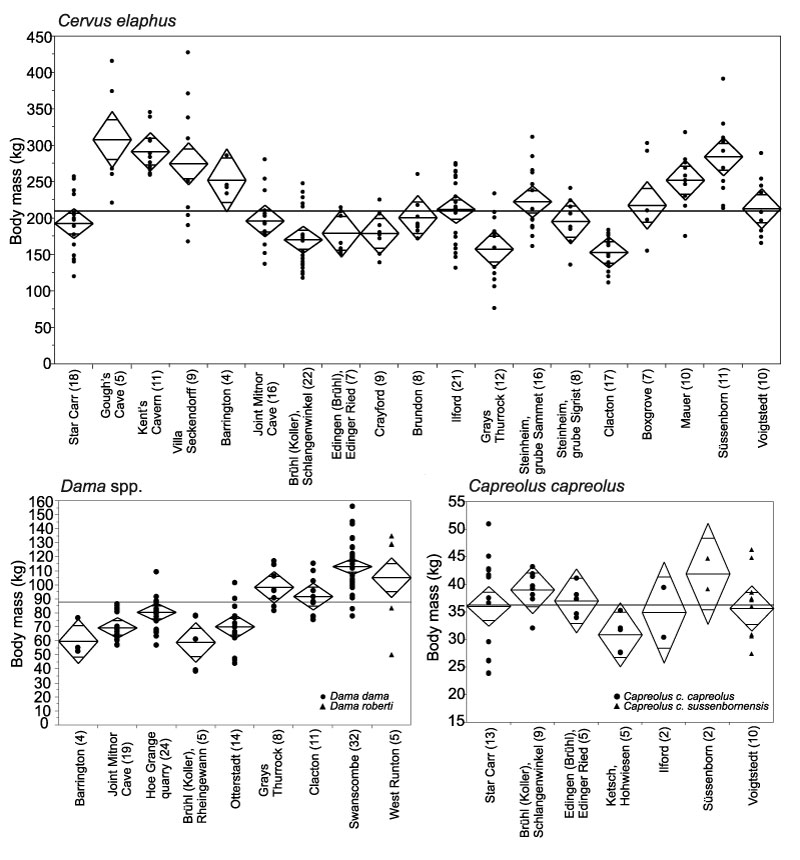
FIGURE 7. Body mass of Megacerini, Rangifer tarandus and Alcini in Middle and Pleistocene localities from Britain and Germany. For explanation of graph, see Figure 6.
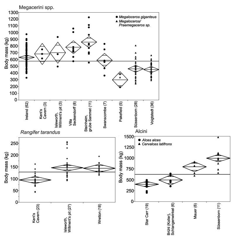
FIGURE 8. Body mass of Rhinocerotidae from Pleistocene localities of Britain and Germany. For explanation of graph, see Figure 6.
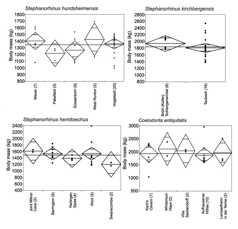
FIGURE 9. Linear regressions of body mass (kg) of Bovidae and Equus ferus/mosbachensis from localities with pollen records, and minimum, maximum and mean NAP % in the pollen records of the localities. Each point represents an individual specimen. Numbers of specimens per each locality are given in brackets after the locality names.
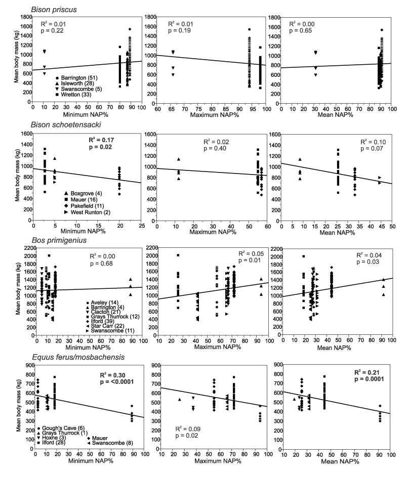
FIGURE 10. Body mass of bovine Bovidae (Bison priscus and Bos primigenius) from Middle and Late Pleistocene localities of Britain and Germany. For explanation of graph, see Figure 6.
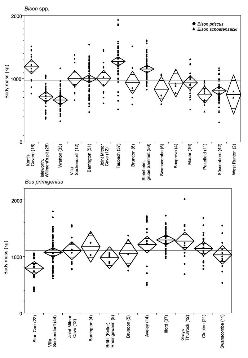
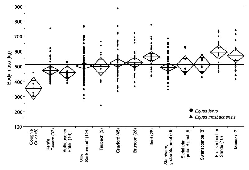
FIGURE 11. Body mass of caballine Equidae (Equus ferus and E. mosbachensis) in Middle and Late Pleistocene localities from Britain and Germany. For explanation of graph, see Figure 6.
 Juha Saarinen. Department of Geosciences and Geography, University of Helsinki, P.O. Box 64, Gustaf Hällströmin katu 2a, 00014 Helsinki, Finland. juha.saarinen@helsinki.fi and Department of Earth Sciences, Natural History Museum, Cromwell Road, London SW7 5BD, UK.
Juha Saarinen is a palaeontologist studying palaeoecology and ecometrics of large herbivorous terrestrial mammals. He received his PhD degree in the University of Helsinki, Finland, in December 2014. In his PhD thesis he examined the evolution of body size in various terrestrial mammal lineages throughout the Cenozoic, as well as variation in diet and body size of Pleistocene European ungulates in relation to environmental conditions. As a part of his work, Juha Saarinen has developed a new palaeodietary analysis method for Proboscidea, based on mesowear of molar teeth. Palaeodietary analyses of ungulates and proboscideans, and their comparison with palaeoenvironmental proxies, mammal community structures and morphological evolution, are the focus of his current research. Juha Saarinen is also the body size data coordinator of the NOW database (http://www.helsinki.fi/science/now).

 Jussi Eronen. Department of Geosciences and Geography, University of Helsinki, P.O. Box 64, Gustaf Hällströmin katu 2a, 00014 Helsinki, Finland. jussi.t.eronen@helsinki.fi
Jussi Eronen is a researcher at the University of Helsinki and at BIOS - an independent research unit, located in Helsinki. He received his PhD in 2006. He aims his research so that the results of the work are relevant for ongoing discussion about the development of and changes in environments and ecosystems, and to the priorities of society. He is a founding member of BIOS (http://bios.fi/), and in the core team of the Scientific Consensus on Maintaining Humanity's Life Support Systems in the 21st Century (http://consensusforaction.stanford.edu/). In general his research agenda is directed towards understanding ecosystem dynamics and climate through time, including present and future. He is Chair of the iCCB (integrative Climate Change Biology, together with Jason Head, (see http://www.iccbio.org/), part of the NECLIME and ETE programmes/communities and an Associate Coordinator for the NOW database (http://www.helsinki.fi/science/now).
 Mikael Fortelius. Department of Geosciences and Geography, University of Helsinki, P.O. Box 64, Gustaf Hällströmin katu 2a, 00014 Helsinki, Finland. mikael.fortelius@helsinki.fi
Mikael Fortelius is a palaeontologist with special interest in the relationships between climate, vegetation and herbivores, especially the plant-eating mammals of the last 25 million years. He has a long-standing interest in how mammalian teeth work, grow, and evolve, and how modelling functional traits can help us understand the past, present, and future states of the world. Mikael Fortelius is Professor of Evolutionary Palaeontology in the Department of Geoscience and Geography at the University of Helsinki and Kristine Bonnevie Professor at the University of Oslo, currently also Alexander von Humboldt Research Awardee at the Museum of Natural History, Berlin. For the last 20 years he has been engaged in developing and coordinating the NOW database of fossil mammals.
 Heikki Seppä. Department of Geosciences and Geography, University of Helsinki, P.O. Box 64, Gustaf Hällströmin katu 2a, 00014 Helsinki, Finland. heikki.seppa@helsinki.fi
Heikki Seppä is a palaeoclimatologist and palaeoecologist interested in Holocene and glacial climate change, theory and methods of quantitative climate reconstructions, and model-proxy comparisons in palaeoclimatology. He is also investigating the influence of past climate changes on species and ecosystems and the impact of early human populations on vegetation.
 Adrian M. Lister. Department of Earth Sciences, Natural History Museum, Cromwell Road, London SW7 5BD, UK. a.lister@nhm.ac.uk
Adrian Lister is a Research Leader in the Department of Earth Sciences of the Natural History Museum in London. He obtained his BA and PhD in Zoology from the University of Cambridge, and from 1991 taught at University College London where he became Professor of Palaeobiology, before moving to the NHM in 2007. His research interests are in the evolution of mammals during the Quaternary ice ages – with special reference to large mammals such as elephants and deer. He has authored nearly 200 scientific papers and his two books on mammoths have sold over 60,000 copies in six languages. Other major research interests include the evolution of endemic island mammals, and the causes of megafaunal extinction at the end of the ice age. As well as his research on fossil mammals, Adrian Lister also studies the taxonomy of their living representatives, serving on the specialist panels of IUCN for both Asian elephants and deer, and has led expeditions to study living elephants in Nepal, India, Ghana and Borneo.
TABLE 1. Localities used in this study with their ages, species analysed and NAP %.
| Locality | Country | Age | Species analysed in this study | Locality used in community-level analyses | Minimum NAP % | Maximum NAP % | Mean NAP % | Reference for age | Reference for pollen record |
| Star Carr | UK | MIS 1 | B. primigenius, C. elaphus, C. capreolus, A. alces | yes | 15.0 | 42.0 | 25.3 | Innes et al., 2011; Penkman et al., 2011 | Clark, 1954 |
| Late-glacial localities (pollen zone III) | Ireland | MIS 2, Allerød-interstadial | M. giganteus | yes | 45.0 | 93.0 | 74.8 | Watts, 1997; Barnosky, 1986 | Watts, 1977 |
| Gough's Cave | UK | MIS 2, Bølling interstadial (GI-1e) | E. ferus, C. elaphus | yes | 89.0 | 94.0 | 91.7 | Currant and Jacobi, 2001; Jacobi and Higham 2009 | Leroi-Gourhan, 1986 |
| Whitemoor Haye | UK | MIS 3 | C. antiquitatis | no | 82.3 | 96.7 | 89.5 | Schreve et al., 2013 | Schreve et al., 2013 |
| Kent's Cavern (cave earth) | UK | MIS 3 | E. ferus, B. priscus, C. elaphus, R. tarandus, M. giganteus, C. antiquitatis | no | Bocherens and Fogel, 1995; Currant and Jacobi, 2001 | ||||
| Isleworth | UK | MIS 5a-d | B. priscus, R. tarandus | no | 86.9 | 94.0 | 90.4 | Penkman et al., 2011; Bates et al., 2014 | Kerney et al., 1982 |
| Wretton (Devensian strata) | UK | MIS 5a-d | B. priscus, R. tarandus | no | 80.0 | 98.0 | 89.0 | Lewin and Gibbard, 2010 | West et al., 1974 |
| Villa Seckendorff | Germany | MIS 5a-d | E. ferus, E. hydruntinus, B. priscus, B. primigenius, C. elaphus, M. giganteus, C. antiquitatis | no | Ziegler, 1996 | ||||
| Aufhausener Höhle | Germany | Last glacial (Würmian) | E. ferus, C. antiquitatis | no | Kley, 1966 | ||||
| Upper Rhine valley localities: Brühl (Koller), Otterstadt, Edingen, Ketsch, Lampertheim in der Tanne | Germany | Late Pleistocene | B. primigenius, C. elaphus, C. capreolus, D. dama, A. alces, S. kirchbergensis, C. antiquitatis | no | Koenigswald and Beug, 1988; Dietrich and Rathgeber, 2012 | ||||
| Reilingen | Germany | MIS 5e? | S. hemitoechus | no | Ziegler and Dean, 1998 | ||||
| Taubach | Germany | MIS 5e | E. ferus, B. priscus, C. elaphus, . capreolus, S. kirchbergensis | no | Brunnacker et al., 1983; van Kolfschoten, 2000 | ||||
| Barrington | UK | MIS 5e | B. priscus, B. primigenius, C. elaphus, D. dama, S. hemitoechus | yes | 89.0 | 94.0 | 91.5 | Ashton et al., 2011 | Gibbard and Stuart, 1982 |
| Joint Mitnor Cave | UK | MIS 5e | B. priscus, C. elaphus, D. dama, S. hemitoechus | no | Ashton et al., 2011 | ||||
| Kirkdale Cave | UK | MIS 5e | B. primigenius | no | Ashton et al., 2011 | ||||
| Hoe Grange quarry | UK | MIS 5e | B. priscus, B. primigenius, D. dama | no | Ashton et al., 2011 | ||||
| Brundon | UK | MIS 7 | E. ferus, B. priscus, B. primigenius | no | Ashton et al., 2011 | ||||
| Ilford | UK | MIS 7 | E. ferus, B. primigenius, C. elaphus, C. capreolus, S. kirchbergensis, S. hemitoechus | yes | 18.0 | 72.0 | 44.6 | Ashton et al., 2011; Penkman et al., 2011 | West et al., 1964 |
| Crayford | UK | MIS 7 | E. ferus, B. primigenius, C. elaphus, S. kirchbergensis, C. antiquitatis | no | Ashton et al., 2011; Penkman et al., 2011 | ||||
| Aveley (zone II B) | UK | MIS 7 | B. primigenius | no | 9.2 | 57.9 | 28.2 | Ashton et al., 2011; Penkman et al., 2011 | West, 1969 |
| Grays Thurrock | UK | MIS 9 | E. ferus, B. primigenius, C. elaphus, D. dama, M. giganteus, S. kirchbergensis | yes | 12.0 | 26.0 | 19.2 | Ashton et al., 2011; Penkman et al., 2011 | Gibbard, 1994 |
| Steinheim a.d. Murr, Grube Sammet | Germany | MIS 10 | E. ferus, B. priscus, B. primigenius, C. elaphus, M. giganteus | yes | Schreve and Bridgland, 2002 | ||||
| Steinheim a.d. Murr, Grube Sigrist | Germany | MIS 11 | E. ferus, C. elaphus | no | Schreve and Bridgland, 2002 | ||||
| Clacton | UK | MIS 11 | E. ferus, B. primigenius, C. elaphus, D. dama, S. hemitoechus | yes | 5.0 | 67.0 | 27.3 | Schreve, 2001; Penkman et al., 2011 | Bridgland et al., 1999 |
| Swanscombe (lower loam) | UK | MIS 11 | E. ferus, B. priscus, B. primigenius, D. dama, M. giganteus, S. hemitoechus | yes | 11.0 | 66.0 | 31.6 | Schreve, 2001; Penkman et al., 2011 | Conway, 1996 |
| Hoxne | UK | MIS 11 | E. ferus, C. elaphus | no | 12.1 | 37.3 | 23.5 | Schreve, 2000; Penkman et al., 2011 | Mullenders, 1993 |
| Frankenbacher Sande | Germany | MIS 11 | E. mosbachensis, B. schoetensacki | no | Van Asperen, 2010 | ||||
| Boxgrove (horizons 5 and 4 c) | UK | MIS 13 | E. ferus, B. schoetensacki, C. elaphus, D. roberti, Megacerini sp., S. hundsheimensis, S. cf. megarhinus | yes | 5.0 | 12.0 | 8.5 | Roberts and Parfitt, 1999 | Roberts, 1986 |
| Pakefield (pollen zone Cr II) | UK | MIS 15 or MIS 17 | B. schoetensacki, S. hundsheimensis | no | 20.0 | 57.0 | 33.3 | Penkman et al., 2011 | West, 1980 |
| Mauer | Germany | MIS 15 | E. mosbachensis, B. schoetensacki, C. elaphus, C. latifrons, S. hundsheimensis | yes | 2.7 | 55.0 | 25.7 | Wagner et al., 2011 | Urban, 1992 |
| Süssenborn | Germany | MIS 16 | E. sussenbornensis, E. altidens, B. schoetensacki, C. elaphus, C. sussenbornensis, C. latifrons, Megacerini sp., S. hundsheimensis | no | Kahlke et al., 2010; Kahlke and Kaiser, 2011 | ||||
| Voigtstedt | Germany | MIS 17 | C. elaphus, C. sussenbornensis, Megacerini sp., S. hundsheimensis | yes | 1.0 | 22.0 | 11.5 | Maul et al., 2007; Kahlke and Kaiser, 2011 | Erd, 1970 |
| West Runton | UK | MIS 17 | Equus sp., B. schoetensacki, C. elaphus, D. cf. roberti, Capreolus sp., Megacerini sp., S. hundsheimensis | yes | 5.0 | 55.0 | 44.6 | Stuart and Lister, 2010; Maul and Parfitt, 2010 | Field and Peglar, 2010 |
TABLE 2. Mean mesowear and body mass values with sample sizes (n) and standard deviations (SD), and minimum, maximum and mean environmental NAP % of the most abundant ungulate species across all localities in which they occur. The species are arranged according to the mean NAP % of their environments from lowest (top) to highest (bottom).
|
Genus |
sp. |
n (mesowear) |
Mean mesowear value |
SD (mesowear) |
Mesowear value range (of locality means) |
n (body mass) |
Mean body mass (kg) |
Body mass range (kg) |
Minimum NAP% |
Maximum NAP% |
Mean NAP% |
| Alces | alces | 8 | 1.00 | 0 | 1.00 | 35 | 433 | 202 - 642 | 12 | 42 | 22 |
| Capreolus | capreolus | 22 | 1.07 | 0.08 | 1.00 - 1.17 | 53 | 35 | 22 - 51 | 12 | 42 | 23 |
| Stephanorhinus | hundsheimensis | 51 | 1.13 | 0.22 | 1.00 - 1.22 | 63 | 1348 | 999 - 1691 | 1 | 57 | 25 |
| Cervalces | latifrons | 13 | 1.11 | 0.16 | 1.00 - 1.23 | 19 | 914 | 593 - 1479 | 3 | 55 | 26 |
| Bison | schoetensacki | 22 | 1.46 | 0.04 | 1.42 - 1.50 | 78 | 835 | 314 - 1313 | 3 | 57 | 28 |
| Stephanorhinus | kirchbergensis | 52 | 1.03 | 0.07 | 1.00 - 1.17 | 25 | 1844 | 1381 - 2538 | 3 | 72 | 30 |
| Cervus | elaphus | 122 | 1.16 | 0.27 | 1.03 - 1.38 | 253 | 211 | 77 - 475 | 1 | 94 | 36 |
| Dama | dama | 42 | 1.12 | 0.08 | 1.04 - 1.17 | 124 | 87 | 39 - 145 | 5 | 94 | 39 |
| Equus | ferus | 174 | 2.35 | 0.29 | 2.00 - 2.45 | 462 | 499 | 301 - 883 | 5 | 94 | 40 |
| Bos | primigenius | 79 | 1.44 | 0.05 | 1.35 - 1.50 | 209 | 1121 | 389 - 2010 | 5 | 94 | 0 |
| Stephanorhinus | hemitoechus | 53 | 1.29 | 0.27 | 1.19 - 1.44 | 25 | 1522 | 1181 - 2384 | 5 | 94 | 49 |
| Megaloceros | giganteus | 48 | 1.38 | 0.22 | 1.10 - 1.69 | 91 | 687 | 329 - 1228 | 11 | 94 | 54 |
| Bison | priscus | 73 | 1.45 | 0.21 | 1.38 - 1.83 | 264 | 1011 | 363 - 1930 | 11 | 94 | 76 |
| Coelodonta | antiquitatis | 35 | 2.21 | 0.65 | 1.33 - 2.53 | 28 | 1905 | 1038 - 2958 | 82 | 97 | 90 |
| Rangifer | tarandus | 17 | 1.09 | 0.19 | 1.09 | 68 | 129 | 43 - 255 | 80 | 98 | 90 |
TABLE 3. Correlations of mean mesowear value of different ungulate groupings with NAP % in the localities. + = significant positive correlation, no = no correlation. Values indicating significant correlations are emboldened.
| Nr. of localities | Correlation | R2 | p | ||
| All ungulates | Min. NAP | 11 | + | 0.47 | 0.02 |
| Max. NAP | 11 | + | 0.67 | 0.002 | |
| Mean NAP | 11 | + | 0.6 | 0.005 | |
| Equidae | Min. NAP | 8 | no | 0.09 | 0.46 |
| Max. NAP | 8 | no | 0.16 | 0.33 | |
| Mean NAP | 9 | no | 0.09 | 0.47 | |
| Bovidae ( Bos and Bison) | Min. NAP | 7 | no | 0.11 | 0.46 |
| Max. NAP | 7 | + | 0.62 | 0.03 | |
| Mean NAP | 8 | no | 0.24 | 0.25 | |
| Cervidae | Min. NAP | 8 | (+) | 0.44 | 0.05 |
| Max. NAP | 8 | + | 0.54 | 0.02 | |
| Mean NAP | 9 | + | 0.58 | 0.02 | |
| Rhinocerotidae | Min. NAP | 8 | + | 0.59 | 0.02 |
| Max. NAP | 8 | + | 0.93 | <0.0001 | |
| Mean NAP | 8 | + | 0.82 | 0.0008 |
TABLE 4. Means comparison of mesowear values of species in the presence/absence of other key ungulate species by paired Wilcoxon tests. M = mean mesowear value. Test statistics (Z and p-values) of the means differences are given for each presence/absence pair for each species (statistically significant values are emboldened). The species presence/absence data per locality were obtained from: Arnold-Bemrose and Newton (1905), Adam (1954), Lister (1984), Ziegler (1996), Schreve (1997), van Kolfschoten (2000) and Currant and Jacobi (2001).
| Cervus elaphus | Equus ferus | Bos primigenius | Bison priscus | Dama dama | Stephanorhinus hemitoechus | |||||||
| M | M | M | M | M | M | |||||||
| A. alces present | 1.26 | Z = 2.14; p = 0.03 | 2.36 | Z = 0;
p = 1 |
1.35 | Z = -2.24; p = 0.02 | 1.34 | Z = -1.51, p = 0.13 | 1.04 | Z = -1.67; p = 0.10 | ||
| A. alces absent | 1.10 | 2.35 | 1.48 | 1.45 | 1.17 | |||||||
| C. capreolus present | 1.26 | Z = 1.46; p = 0.14 | 2.23 | Z = -1.98; p = 0.05 | 1.44 | Z = -1.10; p = 0.27 | 1.38 | Z = -0.97; p = 0.33 | 1.12 | Z = -0.52; p = 0.60 | 1.25 | Z = -1.00; p = 0.32 |
| C. capreolus absent | 1.14 | 2.40 | 1.50 | 1.46 | 1.17 | 1.33 | ||||||
| S. kirchbergensis present | 1.18 | Z = 0.55; p = 0.58 | 2.27 | Z = -1.24; p = 0.22 | 1.45 | Z = -0.56; p = 0.57 | 1.38 | Z = -1.07; p = 0.28 | 1.13 | Z = -0.22; p = 0.83 | 1.25 | Z = -1.00; p = 0.32 |
| S. kirchbergensis absent | 1.14 | 2.38 | 1.48 | 1.46 | 1.14 | 1.33 | ||||||
| Dama dama present | 1.14 | Z = -1.62; p = 0.10 | 2.23 | Z = -1.99; p = 0.05 | 1.41 | Z = -2.05; p = 0.04 | 1.43 | Z = -0.64; p = 0.52 | 1.31 | Z = 1.17; p = 0.24 | ||
| Dama dama absent | 1.28 | 2.40 | 1.50 | 1.45 | 1.19 | |||||||
| Cervus elaphus present | 2.36 | Z = 1.02; p = 0.31 | 1.43 | Z = -0.19; p = 0.85 | ||||||||
| Cervus elaphus absent | 2.28 | 1.44 | ||||||||||
| Bos primigenius present | 1.24 | Z = 1.19; p = 0.24 | 2.33 | Z = -0.81; p = 0.42 | 1.43 | Z = -0.28; p = 0.78 | 1.12 | Z = -0.52; p = 0.60 | 1.30 | Z = 0.49; p = 0.62 | ||
| Bos primigenius absent | 1.14 | 2.42 | 1.43 | 1.17 | 1.25 | |||||||
| S. hemitoechus present | 1.11 | Z = -0.72; p = 0.47 | 2.24 | Z = -1.89; p = 0.06 | 1.45 | Z = -0.59; p = 0.55 | 1.43 | Z = -0.64; p = 0.52 | ||||
| S. hemitoechus absent | 1.19 | 2.41 | 1.50 | 1.45 | ||||||||
| M. giganteus present | 1.15 | Z = -1.57; p = 0.12 | 2.37 | Z = 1.32; p = 0.19 | 1.46 | Z = 0.24; p = 0.81 | 1.43 | Z = -0.19; p = 0.85 | 1.30 | Z = 0.78; p = 0.44 | ||
| M. giganteus absent | 1.32 | 2.28 | 1.44 | 1.44 | 1.20 | |||||||
| R. tarandus present | 1.19 | Z = 0.29; p = 0.67 | 2.41 | Z = 0.88; p = 0.38 | 1.50 | Z = 0.58; p = 0.57 | 1.44 | Z = 0.30; p = 0.77 | ||||
| R. tarandus absent | 1.18 | 2.32 | 1.45 | 1.43 | ||||||||
| B. priscus present | 1.15 | Z = -1.32; p = 0.19 | 2.40 | Z = 2.93; p = 0.003 | 1.48 | Z = 1.00; p = 0.32 | 1.19 | Z = 1.79; p = 0.07 | ||||
| B. priscus absent | 1.27 | 2.19 | 1.44 | 1.06 | ||||||||
| E. ferus present | 1.19 | Z = 0.35; p = 0.72 | 1.46 | Z = 0.24; p = 0.81 | 1.41 | Z = -0.46; p = 0.64 | 1.13 | Z = -0.22; p = 0.83 | 1.25 | Z = -1.00; p = 0.32 | ||
| E. ferus absent | 1.20 | 1.44 | 1.46 | 1.14 | 1.33 | |||||||
| C. antiquitatis present | 1.2 | Z = 1.02; p = 0.31 | 2.41 | Z = 2.18; p = 0.03 | 1.50 | Z = -0.56; p = 0.57 | 1.45 | Z = 0.64; p = 0.52 | ||||
| C. antiquitatis absent | 1.12 | 2.23 | 1.44 | 1.43 | ||||||||
TABLE 5. Pairwise correlations (correlation coefficients from pairwise comparisons) of mean body mass between species, and (bottom three rows) correlation coefficients of species’ mean body mass with minimum, maximum and mean NAP percentages in localities. Correlations based on comparisons of three or more pairs are shown. The pairwise correlations and their p-values are given in Appendix 5. Statistically significant (p <0.05) correlations are emboldened.
| B. priscus | B. scho. | B. prim. | E. ferus | A. alces | C. latifrons | C. elaphus | D. dama | M. giganteus | C. capreolus | R. tarandus | S. kirch. | S. hem. | S. hund. | C. antiq. | |
| Bison priscus | 0.65 | -0.67 | 0.3 | -0.71 | 0.52 | -0.99 | 0.99 | ||||||||
| Bison schoet. | -0.78 | -0.35 | 0.37 | ||||||||||||
| Bos primigenius | 0.65 | 0.62 | -0.08 | 0.18 | -0.4 | 0.89 | |||||||||
| Equus ferus | -0.67 | 0.62 | -0.64 | 0.22 | -0.21 | ||||||||||
| Alces alces | |||||||||||||||
| Cervalces latifrons | -0.78 | 0.76 | |||||||||||||
| Cervus elaphus | -0.35 | -0.08 | -0.64 | 0.76 | -0.07 | -0.91 | -0.98 | -0.75 | -0.41 | ||||||
| Dama dama | -0.71 | 0.22 | -0.07 | -0.93 | |||||||||||
| Meg. giganteus | 0.52 | -0.21 | -0.91 | ||||||||||||
| Capreolus capreolus | -0.4 | -0.98 | |||||||||||||
| Rangifer tarandus | -0.99 | ||||||||||||||
| Steph. kirch. | |||||||||||||||
| Steph. hemit. | 0.99 | 0.89 | -0.75 | -0.93 | |||||||||||
| Steph. hund. | 0.37 | -0.41 | |||||||||||||
| Coelodonta antiquitatis | |||||||||||||||
| Minimum NAP % | -0.06 | -0.64 | 0.1 | -0.89 | 0.55 | -0.91 | 1 | 0.56 | -0.88 | ||||||
| Maximum NAP % | -0.22 | -0.58 | 0.17 | -0.52 | 0.46 | -0.63 | 0.81 | 0.66 | -0.06 | ||||||
| Mean NAP % | -0.11 | -0.82 | 0.18 | -0.78 | 0.61 | -0.82 | 0.92 | 0.66 | 0.07 |
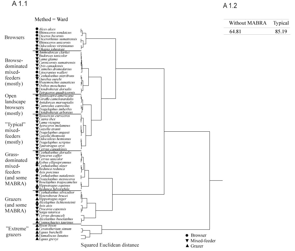
APPENDIX 1.
Statistical tests of univariate mesowear values calculated by our method on the original mesowear data for modern ungulate species (Fortelius and Solounias, 2000). The hierarchical clustering analysis (A 1.1) yielded similar results to the ones shown by Fortelius and Solounias (2000), clustering the species in relatively consistent and biologically meaningful dietary groups, with extreme browsers at one end and extreme grazers at the other. Typical diets in each cluster are named according to those of the dominant species in each cluster. MABRA = ‘”minute abraded brachydonts”; a special case of small ungulates which feed on fruit seeds and acquire a more abrasion-dominated mesowear signal than other browsers because of cusp tip-crushing wear (none of these were present in the Pleistocene of Europe). Discriminant analysis (A 1.2), following the methodology of Fortelius and Solounias (2000) showed that our univariate mesowear values still classify ca. 65 % of all extant ungulate species (excluding MABRA) and 85 % of extant ungulate species “typical of their dietary class” (see Fortelius and Solounias, 2000) correctly into the broad “traditional” dietary classes of “browsers”, “mixed-feeders” and “grazers”.
APPENDIX 2.
Mean mesowear values of species in localities, with standard errors.
APPENDIX 3.
Mean body mass (kg) of all species in localities, with standard errors.
APPENDIX 4.
Pairwise correlation analyses of mean body mass (kg) and mean mesowear of species in localities. Indications of correlation in brackets refer to R2 values, which do not have significant p-values, and ones without brackets refer to to significant correlations. + = positive, ̶ = negative, none = no correlation.
| Genus | species | Correlation | DF | R 2 | p |
| Equus | ferus | none | 11 | 0.001 | 0.91 |
| Stephanorhinus | hemitoechus | (-) | 3 | 0.58 | 0.23 |
| Stephanorhinus | hundsheimensis | (-) | 4 | 0.32 | 0.32 |
| Megaloceros | giganteus | (-) | 2 | 0.96 | 0.13 |
| Dama | dama | none | 3 | 0.001 | 0.9 |
| Coelodonta | antiquitatis | (+) | 2 | 0.99 | 0.07 |
| Cervus | elaphus | none | 8 | 0.05 | 0.54 |
| Bos | primigenius | none | 7 | 0.01 | 0.81 |
| Bison | schoetensacki | - | 3 | 0.98 | 0.001 |
| Bison | priscus | none | 5 | 0.01 | 0.85 |
APPENDIX 5.
Pairwise correlation analyses of mean body mass (kg) between the species (upper rows) and with minimum, maximum and mean NAP % (lower rows) across localities. Count = number of pairs compared. Statistically significant p-values are emboldened.
APPENDIX 6.
Pairwise comparison by Wilcoxon tests of mean body mass of Cervus elaphus in localities. Negative Z values indicate smaller body size and positive values larger body size in the population marked in the first column compared to the one in the second column. Statistically significant p-values are emboldened.
| Fossil population | by Fossil population | Score Mean Difference | Std. Err. Dif. | Z | p |
| Star Carr | Grays Thurrock | 6.04 | 3.28 | 1.84 | 0.07 |
| Star Carr | Brühl (Koller), Schlangenwinkel | 6.77 | 3.71 | 1.82 | 0.07 |
| Star Carr | Ilford | -5.93 | 3.66 | -1.62 | 0.11 |
| Star Carr | Boxgrove | -3.67 | 3.27 | -1.12 | 0.26 |
| Star Carr | Crayford | 3.42 | 3.24 | 1.06 | 0.29 |
| Star Carr | Edingen (Brühl), Edinger Ried | 1.09 | 3.28 | 0.33 | 0.74 |
| Star Carr | Brundon | -0.45 | 3.25 | -0.14 | 0.89 |
| Star Carr | Joint Mitnor Cave | 0.35 | 3.42 | 0.10 | 0.92 |
| Star Carr | Kent's Cavern | -14.43 | 3.26 | -4.43 | <0.0001 |
| Star Carr | Clacton | 10.92 | 3.46 | 3.15 | 0.0016 |
| Star Carr | Mauer | -10.03 | 3.24 | -3.09 | 0.0020 |
| Star Carr | Gough's Cave | -10.35 | 3.43 | -3.02 | 0.0025 |
| Star Carr | Barrington | -8.71 | 3.59 | -2.43 | 0.015 |
| Gough’s Cave | Boxgrove | 3.77 | 2.10 | 1.79 | 0.07 |
| Gough’s Cave | Barrington | 1.58 | 1.84 | 0.86 | 0.39 |
| Gough’s Cave | Clacton | 10.87 | 3.30 | 3.29 | 0.0010 |
| Gough’s Cave | Brühl (Koller), Schlangenwinkel | 12.40 | 3.93 | 3.15 | 0.0016 |
| Gough’s Cave | Crayford | 6.53 | 2.33 | 2.80 | 0.0051 |
| Gough’s Cave | Edingen (Brühl), Edinger Ried | 5.83 | 2.11 | 2.76 | 0.0058 |
| Gough’s Cave | Brundon | 5.69 | 2.22 | 2.56 | 0.010 |
| Kent's Cavern | Gough’s Cave | 0.29 | 2.57 | 0.11 | 0.91 |
| Kent's Cavern | Brühl (Koller), Schlangenwinkel | 16.43 | 3.57 | 4.60 | <0.0001 |
| Kent's Cavern | Clacton | 13.93 | 3.18 | 4.38 | <0.0001 |
| Kent's Cavern | Grays Thurrock | 11.41 | 2.83 | 4.03 | <0.0001 |
| Kent's Cavern | Ilford | 14.27 | 3.49 | 4.09 | <0.0001 |
| Kent's Cavern | Joint Mitnor Cave | 12.66 | 3.11 | 4.07 | <0.0001 |
| Kent's Cavern | Crayford | 9.90 | 2.66 | 3.72 | 0.0002 |
| Kent's Cavern | Brundon | 9.18 | 2.61 | 3.51 | 0.0004 |
| Kent's Cavern | Edingen (Brühl), Edinger Ried | 8.88 | 2.58 | 3.44 | 0.0006 |
| Kent's Cavern | Boxgrove | 5.61 | 2.58 | 2.18 | 0.030 |
| Kent's Cavern | Barrington | 5.28 | 2.61 | 2.02 | 0.043 |
| Villa Seckendorff | Brundon | 4.13 | 2.45 | 1.68 | 0.09 |
| Villa Seckendorff | Steinheim a.d. Murr, grube Sigrist | 4.13 | 2.45 | 1.68 | 0.09 |
| Villa Seckendorff | Ilford | 5.40 | 3.51 | 1.54 | 0.12 |
| Villa Seckendorff | Steinheim a.d. Murr, grube Sammet | 4.43 | 3.07 | 1.44 | 0.15 |
| Villa Seckendorff | Boxgrove | 3.30 | 2.40 | 1.38 | 0.17 |
| Villa Seckendorff | Gough’s Cave | -2.18 | 2.33 | -0.93 | 0.35 |
| Villa Seckendorff | Kent's Cavern | -1.82 | 2.66 | -0.68 | 0.49 |
| Villa Seckendorff | Süssenborn | -1.01 | 2.66 | -0.38 | 0.70 |
| Villa Seckendorff | Barrington | 0.18 | 2.34 | 0.08 | 0.94 |
| Villa Seckendorff | Mauer | 0.11 | 2.59 | 0.04 | 0.97 |
| Villa Seckendorff | Clacton | 12.07 | 3.15 | 3.83 | 0.0001 |
| Villa Seckendorff | Brühl (Koller), Schlangenwinkel | 10.88 | 3.60 | 3.03 | 0.0025 |
| Villa Seckendorff | Grays Thurrock | 8.07 | 2.74 | 2.95 | 0.0032 |
| Villa Seckendorff | Crayford | 6.22 | 2.52 | 2.47 | 0.013 |
| Villa Seckendorff | Edingen (Brühl), Edinger Ried | 5.84 | 2.40 | 2.43 | 0.015 |
| Villa Seckendorff | Star Carr | 7.42 | 3.24 | 2.29 | 0.022 |
| Villa Seckendorff | Joint Mitnor Cave | 6.86 | 3.07 | 2.24 | .025 |
| Joint Mitnor Cave | Crayford | 3.73 | 3.07 | 1.22 | 0.2234 |
| Joint Mitnor Cave | Ilford | -4.35 | 3.59 | -1.21 | 0.2259 |
| Joint Mitnor Cave | Boxgrove | -2.77 | 3.07 | -0.90 | 0.3667 |
| Joint Mitnor Cave | Edingen (Brühl), Edinger Ried | 2.36 | 3.07 | 0.77 | 0.4422 |
| Joint Mitnor Cave | Brundon | -1.03 | 3.06 | -0.34 | 0.7362 |
| Joint Mitnor Cave | Clacton | 12.31 | 3.37 | 3.66 | 0.0003 |
| Joint Mitnor Cave | Gough’s Cave | -9.06 | 3.18 | -2.85 | 0.0044 |
| Joint Mitnor Cave | Barrington | -7.66 | 3.31 | -2.32 | 0.021 |
| Joint Mitnor Cave | Brühl (Koller), Schlangenwinkel | 7.99 | 3.65 | 2.19 | 0.029 |
| Joint Mitnor Cave | Grays Thurrock | 6.27 | 3.14 | 2.00 | 0.046 |
| Brühl (Koller), Schlangenwinkel | Boxgrove | -6.87 | 3.69 | -1.86 | 0.0627 |
| Brühl (Koller), Schlangenwinkel | Barrington | -11.67 | 4.16 | -2.81 | 0.0050 |
| Brühl (Koller), Schlangenwinkel | Brundon | -7.24 | 3.63 | -1.99 | 0.046 |
| Edingen (Brühl), Edinger Ried | Clacton | 5.65 | 3.17 | 1.78 | 0.0753 |
| Edingen (Brühl), Edinger Ried | Boxgrove | -2.57 | 2.23 | -1.15 | 0.2491 |
| Edingen (Brühl), Edinger Ried | Brundon | -2.54 | 2.31 | -1.10 | 0.2716 |
| Edingen (Brühl), Edinger Ried | Brühl (Koller), Schlangenwinkel | 2.45 | 3.69 | 0.66 | 0.5075 |
| Edingen (Brühl), Edinger Ried | Crayford | -0.25 | 2.40 | -0.11 | 0.9157 |
| Edingen (Brühl), Edinger Ried | Barrington | -5.30 | 2.08 | -2.55 | 0.011 |
| Crayford | Brundon | -4.13 | 2.45 | -1.68 | 0.0922 |
| Crayford | Boxgrove | -3.30 | 2.40 | -1.38 | 0.1682 |
| Crayford | Brühl (Koller), Schlangenwinkel | 3.52 | 3.60 | 0.98 | 0.3274 |
| Crayford | Barrington | -6.32 | 2.34 | -2.70 | 0.0069 |
| Crayford | Clacton | 7.82 | 3.15 | 2.48 | 0.013 |
| Brundon | Boxgrove | -1.21 | 2.31 | -0.52 | 0.60 |
| Brundon | Barrington | -4.69 | 2.21 | -2.12 | 0.034 |
| Ilford | Crayford | 6.51 | 3.51 | 1.86 | 0.06 |
| Ilford | Edingen (Brühl), Edinger Ried | 6.29 | 3.59 | 1.75 | 0.08 |
| Ilford | Barrington | -6.10 | 4.02 | -1.52 | 0.13 |
| Ilford | Brundon | 2.50 | 3.54 | 0.71 | 0.48 |
| Ilford | Boxgrove | 0.00 | 3.59 | 0.00 | 1 |
| Ilford | Clacton | 13.31 | 3.63 | 3.67 | 0.0002 |
| Ilford | Brühl (Koller), Schlangenwinkel | 10.52 | 3.83 | 2.75 | 0.0060 |
| Ilford | Grays Thurrock | 9.49 | 3.50 | 2.71 | 0.0067 |
| Ilford | Gough’s Cave | -9.16 | 3.81 | -2.41 | 0.016 |
| Grays Thurrock | Boxgrove | -5.09 | 2.67 | -1.90 | 0.06 |
| Grays Thurrock | Crayford | -2.43 | 2.74 | -0.89 | 0.37 |
| Grays Thurrock | Edingen (Brühl), Edinger Ried | -2.38 | 2.68 | -0.89 | 0.37 |
| Grays Thurrock | Brühl (Koller), Schlangenwinkel | -2.25 | 3.57 | -0.63 | 0.53 |
| Grays Thurrock | Clacton | 1.21 | 3.21 | 0.38 | 0.71 |
| Grays Thurrock | Gough’s Cave | -8.08 | 2.69 | -3.00 | 0.0027 |
| Grays Thurrock | Barrington | -7.50 | 2.75 | -2.73 | 0.0064 |
| Grays Thurrock | Brundon | -5.52 | 2.70 | -2.04 | 0.041 |
| Steinheim a.d. Murr, grube Sammet | Mauer | -5.12 | 3.08 | -1.66 | 0.10 |
| Steinheim a.d. Murr, grube Sammet | Joint Mitnor Cave | 5.44 | 3.32 | 1.64 | 0.10 |
| Steinheim a.d. Murr, grube Sammet | Star Carr | 5.55 | 3.42 | 1.62 | 0.10 |
| Steinheim a.d. Murr, grube Sammet | Brundon | 3.38 | 3.06 | 1.10 | 0.27 |
| Steinheim a.d. Murr, grube Sammet | Barrington | -3.59 | 3.31 | -1.09 | 0.28 |
| Steinheim a.d. Murr, grube Sammet | Ilford | 1.49 | 3.59 | 0.41 | 0.68 |
| Steinheim a.d. Murr, grube Sammet | Boxgrove | 0.82 | 3.07 | 0.27 | 0.79 |
| Steinheim a.d. Murr, grube Sammet | Clacton | 15.10 | 3.37 | 4.49 | <0.0001 |
| Steinheim a.d. Murr, grube Sammet | Kent's Cavern | -10.51 | 3.11 | -3.38 | 0.0007 |
| Steinheim a.d. Murr, grube Sammet | Brühl (Koller), Schlangenwinkel | 11.93 | 3.65 | 3.27 | 0.0011 |
| Steinheim a.d. Murr, grube Sammet | Grays Thurrock | 9.41 | 3.14 | 2.99 | 0.0028 |
| Steinheim a.d. Murr, grube Sammet | Crayford | 7.55 | 3.07 | 2.46 | 0.014 |
| Steinheim a.d. Murr, grube Sammet | Gough’s Cave | -6.96 | 3.18 | -2.19 | 0.029 |
| Steinheim a.d. Murr, grube Sammet | Edingen (Brühl), Edinger Ried | 6.06 | 3.07 | 1.97 | 0.049 |
| Steinheim a.d. Murr, grube Sigrist | Grays Thurrock | 5.10 | 2.70 | 1.89 | 0.06 |
| Steinheim a.d. Murr, grube Sigrist | Brühl (Koller), Schlangenwinkel | 5.20 | 3.63 | 1.43 | 0.15 |
| Steinheim a.d. Murr, grube Sigrist | Steinheim a.d. Murr, grube Sammet | -3.84 | 3.06 | -1.26 | 0.21 |
| Steinheim a.d. Murr, grube Sigrist | Edingen (Brühl), Edinger Ried | 2.54 | 2.31 | 1.10 | 0.27 |
| Steinheim a.d. Murr, grube Sigrist | Crayford | 2.48 | 2.45 | 1.01 | 0.31 |
| Steinheim a.d. Murr, grube Sigrist | Ilford | -3.11 | 3.54 | -0.88 | 0.38 |
| Steinheim a.d. Murr, grube Sigrist | Boxgrove | -0.94 | 2.31 | -0.41 | 0.68 |
| Steinheim a.d. Murr, grube Sigrist | Joint Mitnor Cave | 0.66 | 3.06 | 0.21 | 0.83 |
| Steinheim a.d. Murr, grube Sigrist | Star Carr | 0.45 | 3.25 | 0.14 | 0.89 |
| Steinheim a.d. Murr, grube Sigrist | Brundon | -0.13 | 2.38 | -0.05 | 0.96 |
| Steinheim a.d. Murr, grube Sigrist | Kent's Cavern | -9.39 | 2.61 | -3.59 | 0.0003 |
| Steinheim a.d. Murr, grube Sigrist | Clacton | 9.10 | 3.15 | 2.88 | 0.0039 |
| Steinheim a.d. Murr, grube Sigrist | Mauer | -6.86 | 2.53 | -2.71 | 0.0067 |
| Steinheim a.d. Murr, grube Sigrist | Gough’s Cave | -5.69 | 2.22 | -2.56 | 0.010 |
| Steinheim a.d. Murr, grube Sigrist | Barrington | -5.44 | 2.21 | -2.46 | 0.014 |
| Clacton | Brühl (Koller), Schlangenwinkel | -3.18 | 3.68 | -0.86 | 0.39 |
| Clacton | Brundon | -11.67 | 3.15 | -3.70 | 0.0002 |
| Clacton | Barrington | -10.35 | 3.45 | -3.00 | 0.0027 |
| Clacton | Boxgrove | -8.67 | 3.17 | -2.73 | 0.0063 |
| Boxgrove | Barrington | -2.16 | 2.07 | -1.04 | 0.30 |
| Mauer | Boxgrove | 3.28 | 2.49 | 1.32 | 0.19 |
| Mauer | Gough’s Cave | -2.55 | 2.45 | -1.04 | 0.30 |
| Mauer | Barrington | 0.53 | 2.47 | 0.21 | 0.83 |
| Mauer | Clacton | 12.94 | 3.16 | 4.09 | <0.0001 |
| Mauer | Brühl (Koller), Schlangenwinkel | 13.45 | 3.58 | 3.76 | 0.0002 |
| Mauer | Grays Thurrock | 9.63 | 2.78 | 3.46 | 0.0005 |
| Mauer | Crayford | 8.13 | 2.59 | 3.14 | 0.0017 |
| Mauer | Edingen (Brühl), Edinger Ried | 7.65 | 2.49 | 3.07 | 0.0021 |
| Mauer | Joint Mitnor Cave | 8.53 | 3.08 | 2.77 | 0.0056 |
| Mauer | Kent's Cavern | -6.40 | 2.71 | -2.36 | 0.018 |
| Mauer | Brundon | 5.96 | 2.53 | 2.35 | 0.019 |
| Mauer | Ilford | 7.90 | 3.49 | 2.26 | 0.024 |
| Süssenborn | Mauer | 3.25 | 2.71 | 1.20 | 0.23 |
| Süssenborn | Barrington | 2.90 | 2.61 | 1.11 | 0.27 |
| Süssenborn | Kent's Cavern | -1.09 | 2.77 | -0.39 | 0.69 |
| Süssenborn | Gough’s Cave | -0.87 | 2.57 | -0.34 | 0.73 |
| Süssenborn | Brühl (Koller), Schlangenwinkel | 14.80 | 3.57 | 4.14 | <0.0001 |
| Süssenborn | Clacton | 13.93 | 3.18 | 4.38 | <0.0001 |
| Süssenborn | Grays Thurrock | 11.06 | 2.83 | 3.91 | <0.0001 |
| Süssenborn | Star Carr | 12.67 | 3.26 | 3.89 | 0.0001 |
| Süssenborn | Joint Mitnor Cave | 11.74 | 3.11 | 3.78 | 0.0002 |
| Süssenborn | Crayford | 9.49 | 2.66 | 3.57 | 0.0004 |
| Süssenborn | Edingen (Brühl), Edinger Ried | 8.65 | 2.58 | 3.35 | 0.0008 |
| Süssenborn | Ilford | 11.22 | 3.49 | 3.21 | 0.0013 |
| Süssenborn | Steinheim a.d. Murr, grube Sigrist | 8.31 | 2.61 | 3.18 | 0.0015 |
| Süssenborn | Brundon | 8.10 | 2.61 | 3.10 | 0.0020 |
| Süssenborn | Steinheim a.d. Murr, grube Sammet | 8.82 | 3.11 | 2.84 | 0.0045 |
| Süssenborn | Boxgrove | 6.31 | 2.58 | 2.45 | 0.014 |
| Voigtstedt | Mauer | -5.10 | 2.65 | -1.93 | 0.05 |
| Voigtstedt | Crayford | .96 | 2.59 | 1.92 | 0.06 |
| Voigtstedt | Edingen (Brühl), Edinger Ried | 4.25 | 2.49 | 1.71 | 0.09 |
| Voigtstedt | Villa Seckendorff | -3.91 | 2.59 | -1.51 | 0.13 |
| Voigtstedt | Barrington | -3.33 | 2.47 | -1.34 | 0.18 |
| Voigtstedt | Joint Mitnor Cave | 3.01 | 3.08 | 0.98 | 0.33 |
| Voigtstedt | Star Carr | 2.72 | 3.24 | 0.84 | 0.40 |
| Voigtstedt | Steinheim a.d. Murr, grube Sammet | -2.36 | 3.08 | -0.76 | 0.44 |
| Voigtstedt | Steinheim a.d. Murr, grube Sigrist | 1.46 | 2.53 | 0.58 | 0.56 |
| Voigtstedt | Brundon | 0.79 | 2.53 | 0.31 | 0.76 |
| Voigtstedt | Boxgrove | -0.36 | 2.49 | -0.15 | 0.88 |
| Voigtstedt | Ilford | -0.07 | 3.49 | -0.02 | 0.98 |
| Voigtstedt | Clacton | 11.75 | 3.16 | 3.72 | 0.0002 |
| Voigtstedt | Kent's Cavern | -9.16 | 2.71 | -3.38 | 0.0007 |
| Voigtstedt | Süssenborn | -7.73 | 2.71 | -2.85 | 0.0043 |
| Voigtstedt | Brühl (Koller), Schlangenwinkel | 9.09 | 3.58 | 2.54 | 0.011 |
| Voigtstedt | Grays Thurrock | 6.69 | 2.78 | 2.41 | 0.016 |
| Voigtstedt | Gough’s Cave | -5.55 | 2.45 | -2.27 | 0.024 |
APPENDIX 7.
Pairwise comparison by Wilcoxon tests of mean body mass (kg) of Dama dama in localities.
| Fossil population | by Fossil population | Score Mean Difference | Std. Err. Dif | Z | p |
| Joint Mitnor Cave | Brühl (Koller), Rheingewann | 4.04 | 3.55 | 1.14 | 0.26 |
| Joint Mitnor Cave | Clacton | -12.34 | 3.33 | -3.70 | 0.0002 |
| Joint Mitnor Cave | Grays Thurrock | -11.99 | 3.35 | -3.58 | 0.0003 |
| Joint Mitnor Cave | Hoe Grange quarry | -11.17 | 3.85 | -2.90 | 0.0037 |
| Joint Mitnor Cave | Barrington | 7.41 | 3.73 | 1.99 | 0.047 |
| Hoe Grange quarry | Grays Thurrock | -11.17 | 3.83 | -2.92 | 0.0035 |
| Hoe Grange quarry | Barrington | 11.81 | 4.44 | 2.66 | 0.0078 |
| Hoe Grange quarry | Brühl (Koller), Rheingewann | 10.27 | 4.18 | 2.45 | 0.014 |
| Hoe Grange quarry | Clacton | -7.89 | 3.73 | -2.11 | 0.034 |
| Brühl (Koller), Rheingewann | Barrington | 0.23 | 1.84 | 0.12 | 0.90 |
| Otterstadt | Brühl (Koller), Rheingewann | 3.12 | 2.93 | 1.06 | 0.29 |
| Otterstadt | Barrington | 3.05 | 3.03 | 1.01 | 0.31 |
| Otterstadt | Joint Mitnor Cave | 1.24 | 3.41 | 0.36 | 0.72 |
| Otterstadt | Grays Thurrock | -9.23 | 2.88 | -3.21 | 0.0013 |
| Otterstadt | Clacton | -8.77 | 2.96 | -2.96 | 0.0031 |
| Otterstadt | Hoe Grange quarry | -7.86 | 3.74 | -2.10 | 0.035 |
| Grays Thurrock | Clacton | 2.70 | 2.61 | 1.03 | 0.30 |
| Grays Thurrock | Brühl (Koller), Rheingewann | 6.34 | 2.22 | 2.85 | 0.0043 |
| Grays Thurrock | Barrington | 5.81 | 2.21 | 2.63 | 0.0085 |
| Swanscombe | Hoe Grange quarry | 24.97 | 4.40 | 5.67 | <0.0001 |
| Swanscombe | Joint Mitnor Cave | 24.62 | 4.31 | 5.72 | <0.0001 |
| Swanscombe | Otterstadt | 21.56 | 4.30 | 5.01 | <0.0001 |
| Swanscombe | Brühl (Koller), Rheingewann | 18.15 | 5.21 | 3.49 | 0.0005 |
| Swanscombe | Clacton | 14.78 | 4.39 | 3.37 | 0.0008 |
| Swanscombe | Barrington | 17.86 | 5.59 | 3.20 | 0.0014 |
| Swanscombe | Grays Thurrock | 10.31 | 4.62 | 2.23 | 0.026 |
| West Runton | Otterstadt. Otterstadtler Altrhein (Oberrhein) | 5.56 | 2.93 | 1.90 | 0.06 |
| West Runton | Brühl (Koller), Rheingewann (Oberrhein) | 3.60 | 1.91 | 1.88 | 0.06 |
| West Runton | Joint Mitnor Cave | 6.06 | 3.55 | 1.71 | 0.09 |
| West Runton | Hoe Grange quarry | 6.16 | 4.18 | 1.47 | 0.14 |
| West Runton | Barrington | 2.48 | 1.84 | 1.35 | 0.18 |
| West Runton | Clacton | 2.33 | 2.57 | 0.91 | 0.36 |
| West Runton | Grays Thurrock | 1.46 | 2.22 | 0.66 | 0.51 |
| West Runton | Swanscombe | 1.04 | 5.21 | 0.20 | 0.84 |
APPENDIX 8.
Pairwise comparison by Wilcoxon tests of mean body mass (kg) of Capreolus sp. in localities.
| Fossil population | by Fossil population | Score Mean Difference | Std. Err. Dif. | Z | p |
| Star Carr | Ketsch, Hohwiesen | 2.49 | 2.81 | 0.89 | 0.38 |
| Star Carr | Brühl (Koller), Schlangenwinkel | -1.50 | 2.82 | -0.53 | 0.59 |
| Star Carr | Edingen (Brühl), Edinger Ried | 0.55 | 2.81 | 0.20 | 0.84 |
| Star Carr | Ilford | 0.29 | 3.40 | 0.08 | 0.93 |
| Edingen (Brühl), Edinger Ried | Brühl (Koller), Schlangenwinkel | -2.96 | 2.33 | -1.27 | 0.20 |
| Ketsch, Hohwiesen | Ilford | -1.05 | 1.81 | -0.58 | 0.56 |
| Ketsch, Hohwiesen | Brühl (Koller), Schlangenwinkel | -6.22 | 2.33 | -2.67 | 0.0077 |
| Ketsch, Hohwiesen | Edingen (Brühl), Edinger Ried | -4.00 | 1.91 | -2.09 | 0.037 |
| Ilford | Brühl (Koller), Schlangenwinkel | -2.14 | 2.59 | -0.82 | 0.41 |
| Ilford | Edingen (Brühl), Edinger Ried | -0.35 | 1.81 | -0.19 | 0.85 |
| Süssenborn | Ketsch, Hohwiesen | 3.15 | 1.81 | 1.74 | 0.08 |
| Süssenborn | Edingen (Brühl), Edinger Ried | 2.45 | 1.81 | 1.36 | 0.18 |
| Süssenborn | Brühl (Koller), Schlangenwinkel | 2.14 | 2.59 | 0.82 | 0.41 |
| Süssenborn | Star Carr | 2.60 | 3.40 | 0.76 | 0.44 |
| Süssenborn | Ilford | 0.50 | 1.29 | 0.39 | 0.70 |
| Voigtstedt | Brühl (Koller), Schlangenwinkel | -3.91 | 2.58 | -1.51 | 0.13 |
| Voigtstedt | Süssenborn | -3.30 | 2.79 | -1.18 | 0.24 |
| Voigtstedt | Ketsch, Hohwiesen | 2.55 | 2.45 | 1.04 | 0.30 |
| Voigtstedt | Edingen (Brühl), Edinger Ried | -1.05 | 2.45 | -0.43 | 0.67 |
| Voigtstedt | Ilford | 0.00 | 2.79 | 0.00 | 1.00 |
| Voigtstedt | Star Carr | 0.00 | 2.85 | 0.00 | 1.00 |
APPENDIX 9.
Pairwise comparison by Wilcoxon tests of mean body mass (kg) of Megacerini spp. in localities. The significant differences are mostly due to the smaller size of early Middle Pleistocene Praemegaceros and Megaloceros species compared to late Middle and Late Pleistocene Megaloceros giganteus.
| Fossil population | by Fossil population | Score Mean Difference | Std. Err. Dif. | Z | p |
| Kent's Cavern | Ireland | 7.86 | 11.18 | 0.70 | 0.48 |
| Kent's Cavern | Isleworth, Willment’s pit | 0.00 | 1.53 | 0.00 | 1.00 |
| Isleworth, Willment’s pit | Ireland | 5.77 | 11.18 | 0.52 | 0.61 |
| Villa Seckendorff | Swanscombe | 4.42 | 2.31 | 1.91 | 0.06 |
| Villa Seckendorff | Kent's Cavern | 2.06 | 2.25 | 0.92 | 0.36 |
| Villa Seckendorff | Isleworth, Willment’s pit | 1.60 | 2.25 | 0.71 | 0.48 |
| Villa Seckendorff | Steinheim, grube Sammet | -1.84 | 2.61 | -0.70 | 0.48 |
| Villa Seckendorff | Süssenborn | 15.99 | 4.22 | 3.79 | 0.0002 |
| Villa Seckendorff | Pakefield | 6.34 | 2.22 | 2.85 | 0.0043 |
| Villa Seckendorff | Ireland | 17.01 | 7.65 | 2.22 | 0.026 |
| Steinheim, grube Sammet | Kent's Cavern | 4.24 | 2.72 | 1.56 | 0.12 |
| Steinheim, grube Sammet | Isleworth, Willment’s pit | 3.39 | 2.72 | 1.25 | 0.21 |
| Steinheim, grube Sammet | Ireland | 22.85 | 6.94 | 3.29 | 0.0010 |
| Steinheim, grube Sammet | Pakefield | 7.85 | 2.57 | 3.06 | 0.0022 |
| Swanscombe | Kent's Cavern | -2.38 | 2.09 | -1.14 | 0.25 |
| Swanscombe | Isleworth, Willment’s pit | -1.43 | 2.09 | -0.68 | 0.49 |
| Swanscombe | Ireland | -5.17 | 8.00 | -0.65 | 0.52 |
| Swanscombe | Pakefield | 5.14 | 2.11 | 2.44 | 0.015 |
| Swanscombe | Steinheim, grube Sammet | -5.84 | 2.58 | -2.26 | 0.024 |
| Pakefield | Ireland | -32.74 | 9.06 | -3.61 | 0.0003 |
| Pakefield | Isleworth, Willment’s pit | -3.73 | 1.79 | -2.09 | 0.037 |
| Pakefield | Kent's Cavern | -3.73 | 1.79 | -2.09 | 0.037 |
| Süssenborn | Swanscombe | -8.48 | 4.33 | -1.96 | 0.05 |
| Süssenborn | Ireland | -27.68 | 5.95 | -4.65 | <0.0001 |
| Süssenborn | Steinheim, grube Sammet | -18.04 | 4.06 | -4.45 | <0.0001 |
| Süssenborn | Pakefield | 11.67 | 4.69 | 2.49 | 0.013 |
| Süssenborn | Kent's Cavern | -13.10 | 5.52 | -2.37 | 0.018 |
| Süssenborn | Isleworth, Willment’s pit | -11.26 | 5.52 | -2.04 | 0.042 |
| Voigtstedt | Süssenborn | -0.79 | 4.69 | -0.17 | 0.87 |
| Voigtstedt | Ireland | -34.80 | 5.96 | -5.84 | <0.0001 |
| Voigtstedt | Steinheim, grube Sammet | -22.85 | 4.72 | -4.84 | <0.0001 |
| Voigtstedt | Villa Seckendorff | -21.16 | 5.02 | -4.21 | <0.0001 |
| Voigtstedt | Kent's Cavern | -18.96 | 6.85 | -2.77 | 0.0057 |
| Voigtstedt | Pakefield | 15.15 | 5.72 | 2.65 | 0.0081 |
| Voigtstedt | Swanscombe | -11.86 | 5.19 | -2.29 | 0.022 |
| Voigtstedt | Isleworth, Willment’s pit | -14.63 | 6.85 | -2.13 | 0.033 |
APPENDIX 10.
Pairwise comparison by Wilcoxon tests of mean body mass (kg) of Rangifer tarandus in localities.
| Fossil population | by Fossil population | Score Mean Difference | Std. Err. Dif. | Z | p |
| Kent's Cavern | Isleworth, Willment's pit | -17.67 | 4.14 | -4.27 | <0.0001 |
| Wretton | Kent's Cavern | 17.53 | 3.77 | 4.65 | <0.0001 |
| Wretton | Isleworth, Willment's pit | 3.06 | 4.00 | 0.76 | 0.44 |
APPENDIX 11.
Pairwise comparison by Wilcoxon tests of mean body mass (kg) of Alcini in localities. The significant differences are mostly due to the larger size of early Middle Pleistocene Cervalces latifrons compared to Late Pleistocene and Holocene Alces alces.
| Fossil population | by Fossil population | Score Mean Difference | Std. Err. Dif. | Z | p |
| Star Carr | Mauer | -12.39 | 3.45 | -3.60 | 0.0003 |
| Star Carr | Brühl (Koller), Schlangenwinkel | -6.47 | 3.45 | -1.88 | 0.061 |
| Mauer | Brühl (Koller), Schlangenwinkel | 5.17 | 2.08 | 2.48 | 0.013 |
| Süssenborn | Star Carr | 14.93 | 3.34 | 4.48 | <0.0001 |
| Süssenborn | Brühl (Koller), Schlangenwinkel | 8.37 | 2.56 | 3.27 | 0.0011 |
| Süssenborn | Mauer | 5.54 | 2.56 | 2.16 | 0.031 |
APPENDIX 12.
Pairwise comparison by Wilcoxon tests of mean body mass (kg) of Stephanorhinus hundsheimensis in localities.
| Fossil population | by Fossil population | Score Mean Difference | Std. Err. Dif. | Z | p |
| Pakefield | Mauer | -3.33 | 2.09 | -1.60 | 0.11 |
| Süssenborn | Mauer | -2.63 | 2.17 | -1.21 | 0.22 |
| Süssenborn | Pakefield | 0.25 | 1.94 | 0.13 | 0.90 |
| West Runton | Süssenborn | 1.67 | 2.00 | 0.83 | 0.40 |
| West Runton | Pakefield | 0.42 | 1.44 | 0.29 | 0.77 |
| West Runton | Mauer | 0.32 | 2.20 | 0.15 | 0.88 |
| Voigtstedt | Pakefield | 7.48 | 4.20 | 1.78 | 0.08 |
| Voigtstedt | Süssenborn | 3.36 | 3.56 | 0.94 | 0.35 |
| Voigtstedt | Mauer | -1.06 | 3.49 | -0.30 | 0.76 |
| Voigtstedt | West Runton | -1.38 | 4.82 | -0.29 | 0.78 |
APPENDIX 13.
Pairwise comparison by Wilcoxon tests of mean body mass (kg) of Stephanorhinus hemitoechus in localities.
| Fossil population | by Fossil population | Score Mean Difference | Std. Err. Dif. | Z | p |
| Joint Mitnor Cave | Ilford | 2.19 | 2.39 | 0.91 | 0.36 |
| Joint Mitnor Cave | Barrington | 1.53 | 2.59 | 0.59 | 0.56 |
| Reilingen, Spies | Joint Mitnor Cave | -2.63 | 1.62 | -1.62 | 0.11 |
| Reilingen, Spies | Barrington | -3.43 | 2.34 | -1.47 | 0.14 |
| Reilingen, Spies | Ilford | -0.19 | 2.21 | -0.08 | 0.93 |
| Ilford | Barrington | -1.53 | 2.45 | -0.63 | 0.53 |
| Swanscombe | Barrington | -4.58 | 2.59 | -1.77 | 0.08 |
| Swanscombe | Reilingen, Spies | -2.63 | 1.62 | -1.62 | 0.11 |
| Swanscombe | Ilford | -3.44 | 2.39 | -1.44 | 0.15 |
| Swanscombe | Joint Mitnor Cave | -1.50 | 1.29 | -1.16 | 0.25 |
APPENDIX 14.
Pairwise comparison by Wilcoxon tests of mean body mass (kg) of Coelodonta antiquitatis in localities.
| Fossil population | by Fossil population | Score Mean Difference | Std. Err. Dif. | Z | p |
| Kent's Cavern | Aufhausener höhle | 2.31 | 2.49 | 0.93 | 0.35 |
| Whitemoor Haye | Aufhausener höhle | 3.30 | 2.79 | 1.18 | 0.24 |
| Whitemoor Haye | Kent's Cavern | 1.61 | 2.20 | 0.73 | 0.46 |
| Whitemoor Haye | Lampertheim in der Tanne | 0.42 | 1.44 | 0.29 | 0.77 |
| Villa Seckendorff | Aufhausener höhle | 3.30 | 2.79 | 1.18 | 0.24 |
| Villa Seckendorff | Lampertheim in der Tanne | 0.42 | 1.44 | 0.29 | 0.77 |
| Villa Seckendorff | Kent's Cavern | -0.32 | 2.20 | -0.15 | 0.88 |
| Villa Seckendorff | Whitemoor Haye | 0.00 | 1.29 | 0.00 | 1.00 |
| Lampertheim in der Tanne | Aufhausener höhle | 0.65 | 2.56 | 0.25 | 0.80 |
| Lampertheim in der Tanne | Kent's Cavern | 0.00 | 2.09 | 0.00 | 1.00 |
APPENDIX 15.
Pairwise comparison by Wilcoxon tests of mean body mass (kg) of Bison priscus/schoetensacki in localities. Some of the significant differences are due to the smaller size of early Middle Pleistocene Bison schoetensacki compared to Late Pleistocene B. priscus.
| Fossil population | by Fossil population | Score Mean Difference | Std. Err. Dif. | Z | p |
| Kent's Cavern | Boxgrove | 6.41 | 3.31 | 1.94 | 0.053 |
| Kent's Cavern | Brundon | 5.16 | 3.11 | 1.66 | 0.097 |
| Kent's Cavern | Joint Mitnor Cave | 5.18 | 3.14 | 1.65 | 0.099 |
| Kent's Cavern | Isleworth, Willment’s pit | 19.59 | 4.03 | 4.87 | <0.0001 |
| Kent's Cavern | Barrington | 14.33 | 5.58 | 2.57 | 0.010 |
| Isleworth, Willment’s pit | Brundon | -6.38 | 4.48 | -1.42 | 0.16 |
| Isleworth, Willment’s pit | Barrington | -24.42 | 5.40 | -4.53 | <0.0001 |
| Isleworth, Willment’s pit | Boxgrove | -10.71 | 5.01 | -2.14 | 0.033 |
| Wretton | Swanscombe | -8.52 | 5.33 | -1.60 | 0.11 |
| Wretton | Pakefield | -6.67 | 4.47 | -1.49 | 0.14 |
| Wretton | Isleworth, Willment’s pit | -5.31 | 4.56 | -1.17 | 0.24 |
| Wretton | West Runton | -7.69 | 7.46 | -1.03 | 0.303 |
| Wretton | Barrington | -30.00 | 5.45 | -5.50 | <0.0001 |
| Wretton | Kent's Cavern | -22.78 | 4.35 | -5.23 | <0.0001 |
| Wretton | Steinheim, grube Sammet | -42.07 | 5.67 | -7.42 | <0.0001 |
| Wretton | Taubach | -31.07 | 4.87 | -6.38 | <0.0001 |
| Wretton | Villa Seckendorff | -16.88 | 4.43 | -3.81 | 0.0001 |
| Wretton | Mauer | -16.33 | 4.35 | -3.75 | 0.0002 |
| Wretton | Joint Mitnor Cave | -15.97 | 4.43 | -3.61 | 0.0003 |
| Wretton | Süssenborn | -16.45 | 5.07 | -3.24 | 0.0012 |
| Wretton | Boxgrove | -14.44 | 5.73 | -2.52 | 0.012 |
| Wretton | Brundon | -10.93 | 5.06 | -2.16 | 0.031 |
| Villa Seckendorff | Kent's Cavern | -5.32 | 3.14 | -1.69 | 0.09 |
| Villa Seckendorff | Swanscombe | 3.83 | 2.69 | 1.42 | 0.16 |
| Villa Seckendorff | West Runton | 4.38 | 3.20 | 1.37 | 0.17 |
| Villa Seckendorff | Brundon | 2.13 | 2.67 | 0.80 | 0.43 |
| Villa Seckendorff | Mauer | 1.82 | 3.14 | 0.58 | 0.56 |
| Villa Seckendorff | Barrington | 0.41 | 5.88 | 0.07 | 0.94 |
| Villa Seckendorff | Boxgrove | 0.17 | 2.75 | 0.06 | 0.95 |
| Villa Seckendorff | Joint Mitnor Cave | -0.08 | 2.89 | -0.03 | 0.98 |
| Villa Seckendorff | Isleworth, Willment’s pit | 13.04 | 4.03 | 3.23 | 0.0012 |
| Villa Seckendorff | Taubach | -12.25 | 4.75 | -2.58 | 0.0099 |
| Villa Seckendorff | Pakefield | 6.19 | 2.83 | 2.18 | 0.029 |
| Villa Seckendorff | Süssenborn | 11.20 | 5.15 | 2.17 | 0.030 |
| Villa Seckendorff | Steinheim, grube Sammet | -13.56 | 6.29 | -2.16 | 0.031 |
| Joint Mitnor Cave | Brundon | 1.38 | 2.67 | 0.52 | 0.61 |
| Joint Mitnor Cave | Boxgrove | 0.83 | 2.75 | 0.30 | 0.76 |
| Joint Mitnor Cave | Barrington | -0.15 | 5.88 | -0.03 | 0.98 |
| Joint Mitnor Cave | Isleworth, Willment’s pit | 11.13 | 4.03 | 2.76 | 0.0058 |
| Taubach | Kent's Cavern | 5.28 | 4.62 | 1.14 | 0.25 |
| Taubach | Barrington | 23.39 | 5.52 | 4.24 | <0.0001 |
| Taubach | Isleworth, Willment’s pit | 27.89 | 4.74 | 5.89 | <0.0001 |
| Taubach | Pakefield | 20.40 | 4.81 | 4.24 | <0.0001 |
| Taubach | Süssenborn | 31.34 | 5.17 | 6.06 | <0.0001 |
| Taubach | Mauer | 16.79 | 4.62 | 3.63 | 0.0003 |
| Taubach | Swanscombe | 15.89 | 5.85 | 2.72 | 0.0066 |
| Taubach | Steinheim, grube Sammet | 14.07 | 5.72 | 2.46 | 0.014 |
| Taubach | Joint Mitnor Cave | 11.31 | 4.75 | 2.38 | 0.017 |
| Taubach | Boxgrove | 14.27 | 6.30 | 2.26 | 0.024 |
| Taubach | Brundon | 10.94 | 5.53 | 1.98 | 0.048 |
| Brundon | Barrington | -5.31 | 7.16 | -0.74 | 0.46 |
| Brundon | Boxgrove | -0.63 | 1.95 | -0.32 | 0.75 |
| Steinheim, grube Sammet | Joint Mitnor Cave | 10.98 | 6.29 | 1.75 | 0.081 |
| Steinheim, grube Sammet | Kent's Cavern | -4.58 | 5.93 | -0.77 | 0.44 |
| Steinheim, grube Sammet | Isleworth, Willment’s pit | 38.46 | 5.65 | 6.81 | <0.0001 |
| Steinheim, grube Sammet | Pakefield | 31.05 | 6.43 | 4.83 | <0.0001 |
| Steinheim, grube Sammet | Brundon | 15.22 | 7.75 | 1.96 | 0.050 |
| Steinheim, grube Sammet | Mauer | 18.48 | 5.93 | 3.12 | 0.0018 |
| Steinheim, grube Sammet | Barrington | 17.63 | 6.01 | 2.93 | 0.0033 |
| Steinheim, grube Sammet | Boxgrove | 20.49 | 9.04 | 2.27 | 0.023 |
| Swanscombe | Barrington | -10.76 | 7.64 | -1.41 | 0.16 |
| Swanscombe | Joint Mitnor Cave | -3.26 | 2.69 | -1.21 | 0.23 |
| Swanscombe | Isleworth, Willment’s pit | 5.30 | 4.69 | 1.13 | 0.26 |
| Swanscombe | Boxgrove | -1.58 | 1.84 | -0.86 | 0.39 |
| Swanscombe | Mauer | -2.23 | 3.18 | -0.70 | 0.48 |
| Swanscombe | Pakefield | 1.75 | 2.57 | 0.68 | 0.50 |
| Swanscombe | Brundon | -0.55 | 2.01 | -0.27 | 0.78 |
| Swanscombe | Kent's Cavern | -8.27 | 3.18 | -2.60 | 0.0093 |
| Swanscombe | Steinheim, grube Sammet | -20.70 | 8.29 | -2.50 | 0.013 |
| Boxgrove | Barrington | -6.07 | 8.32 | -0.73 | 0.47 |
| Mauer | Barrington | -4.89 | 5.58 | -0.88 | 0.38 |
| Mauer | Joint Mitnor Cave | -1.68 | 3.14 | -0.53 | 0.59 |
| Mauer | Brundon | 1.03 | 3.11 | 0.33 | 0.74 |
| Mauer | Boxgrove | 0.00 | 3.31 | 0.00 | 1.000 |
| Mauer | Isleworth, Willment’s pit | 11.83 | 4.03 | 2.94 | 0.0033 |
| Mauer | Kent's Cavern | -8.69 | 3.32 | -2.62 | 0.0088 |
| Pakefield | Boxgrove | -3.92 | 2.61 | -1.50 | 0.133 |
| Pakefield | Brundon | -2.70 | 2.56 | -1.06 | 0.29 |
| Pakefield | Isleworth, Willment’s pit | 1.84 | 4.06 | 0.45 | 0.65 |
| Pakefield | Kent's Cavern | -12.04 | 3.11 | -3.87 | 0.0001 |
| Pakefield | Barrington | -18.57 | 6.00 | -3.10 | 0.0020 |
| Pakefield | Mauer | -7.13 | 3.11 | -2.29 | 0.022 |
| Pakefield | Joint Mitnor Cave | -5.84 | 2.83 | -2.06 | 0.039 |
| Süssenborn | Mauer | -9.49 | 4.96 | -1.91 | 0.056 |
| Süssenborn | Isleworth, Willment’s pit | 9.02 | 4.97 | 1.82 | 0.069 |
| Süssenborn | Boxgrove | -8.90 | 7.02 | -1.27 | 0.21 |
| Süssenborn | Pakefield | 5.79 | 5.23 | 1.11 | 0.27 |
| Süssenborn | Brundon | -3.33 | 6.11 | -0.55 | 0.59 |
| Süssenborn | Swanscombe | -1.01 | 6.49 | -0.16 | 0.88 |
| Süssenborn | Kent's Cavern | -23.00 | 4.96 | -4.64 | <0.0001 |
| Süssenborn | Steinheim, grube Sammet | -38.83 | 5.80 | -6.69 | <0.0001 |
| Süssenborn | Barrington | -20.84 | 5.62 | -3.71 | 0.0002 |
| Süssenborn | Joint Mitnor Cave | -10.98 | 5.15 | -2.13 | 0.033 |
| West Runton | Taubach | -16.07 | 8.28 | -1.94 | 0.05 |
| West Runton | Barrington | -15.85 | 11.13 | -1.42 | 0.16 |
| West Runton | Mauer | -4.78 | 4.00 | -1.19 | 0.23 |
| West Runton | Boxgrove | -1.88 | 1.62 | -1.16 | 0.25 |
| West Runton | Joint Mitnor Cave | -3.21 | 3.20 | -1.00 | 0.32 |
| West Runton | Brundon | -1.00 | 2.00 | -0.50 | 0.62 |
| West Runton | Süssenborn | -3.93 | 9.30 | -0.42 | 0.67 |
| West Runton | Swanscombe | -0.35 | 1.81 | -0.19 | 0.85 |
| West Runton | Isleworth, Willment’s pit | 0.80 | 6.44 | 0.12 | 0.90 |
| West Runton | Pakefield | 0.00 | 2.99 | 0.00 | 1.000 |
| West Runton | Steinheim, grube Sammet | -28.74 | 12.15 | -2.37 | 0.018 |
| West Runton | Kent's Cavern | -8.16 | 4.00 | -2.04 | 0.042 |
APPENDIX 16.
Pairwise comparison by Wilcoxon tests of mean body mass (kg) of Bos primigenius in localities.
| Fossil population | by Fossil population | Score Mean Difference | Std. Err. Dif. | Z | p |
| Star Carr | Brundon | -6.63 | 3.93 | -1.69 | 0.092 |
| Star Carr | Clacton | -15.03 | 3.83 | -3.92 | <0.0001 |
| Star Carr | Ilford | -28.83 | 4.73 | -6.09 | <0.0001 |
| Star Carr | Grays Thurrock | -13.07 | 3.57 | -3.66 | 0.0003 |
| Star Carr | Joint Mitnor Cave | -9.98 | 3.57 | -2.79 | 0.0052 |
| Star Carr | Aveley | -9.18 | 3.60 | -2.55 | 0.011 |
| Star Carr | Barrington | -10.19 | 4.16 | -2.45 | 0.014 |
| Star Carr | Brühl (Koller), Rheingewann | -7.93 | 3.63 | -2.18 | 0.029 |
| Villa Seckendorff | Grays Thurrock | -9.60 | 5.31 | -1.81 | 0.071 |
| Villa Seckendorff | Aveley | -5.98 | 5.18 | -1.15 | 0.25 |
| Villa Seckendorff | Clacton | -4.99 | 5.01 | -1.00 | 0.32 |
| Villa Seckendorff | Barrington | -5.86 | 7.31 | -0.80 | 0.42 |
| Villa Seckendorff | Brühl (Koller), Rheingewann | 3.62 | 5.82 | 0.62 | 0.53 |
| Villa Seckendorff | Joint Mitnor Cave | -2.28 | 5.31 | -0.43 | 0.67 |
| Villa Seckendorff | Swanscombe | 1.25 | 5.40 | 0.23 | 0.82 |
| Villa Seckendorff | Brundon | -0.11 | 6.74 | -0.02 | 0.99 |
| Villa Seckendorff | Ilford | -18.79 | 5.30 | -3.54 | 0.0004 |
| Villa Seckendorff | Star Carr | 16.13 | 5.01 | 3.22 | 0.0013 |
| Joint Mitnor Cave | Grays Thurrock | -3.00 | 2.89 | -1.04 | 0.30 |
| Joint Mitnor Cave | Brühl (Koller), Rheingewann | 2.19 | 2.70 | 0.81 | 0.42 |
| Joint Mitnor Cave | Aveley | -2.24 | 3.01 | -0.75 | 0.46 |
| Joint Mitnor Cave | Barrington | -1.50 | 2.75 | -0.55 | 0.59 |
| Joint Mitnor Cave | Clacton | -1.51 | 3.50 | -0.43 | 0.67 |
| Joint Mitnor Cave | Brundon | 0.99 | 2.69 | 0.37 | 0.71 |
| Joint Mitnor Cave | Ilford | -10.13 | 4.91 | -2.07 | 0.040 |
| Barrington | Aveley | -1.45 | 3.03 | -0.48 | 0.63 |
| Brühl (Koller), Rheingewann | Barrington | -2.81 | 2.21 | -1.27 | 0.20 |
| Brühl (Koller), Rheingewann | Aveley | -3.04 | 2.88 | -1.06 | 0.29 |
| Brühl (Koller), Rheingewann | Brundon | -0.49 | 2.22 | -0.22 | 0.83 |
| Brundon | Aveley | -1.76 | 2.93 | -0.60 | 0.55 |
| Brundon | Barrington | -0.68 | 1.84 | -0.37 | 0.71 |
| Ilford | Brundon | 11.73 | 6.10 | 1.92 | 0.055 |
| Ilford | Barrington | 7.58 | 6.59 | 1.15 | 0.25 |
| Ilford | Aveley | -1.02 | 4.81 | -0.21 | 0.83 |
| Ilford | Grays Thurrock | 0.82 | 4.91 | 0.17 | 0.87 |
| Ilford | Brühl (Koller), Rheingewann | 20.71 | 5.32 | 3.89 | <0.0001 |
| Ilford | Clacton | 11.06 | 4.73 | 2.34 | 0.019 |
| Grays Thurrock | Brundon | 2.98 | 2.69 | 1.11 | 0.27 |
| Grays Thurrock | Clacton | 3.08 | 3.50 | 0.88 | 0.38 |
| Grays Thurrock | Barrington | 1.17 | 2.75 | 0.42 | 0.67 |
| Grays Thurrock | Aveley | -0.23 | 3.01 | -0.08 | 0.94 |
| Grays Thurrock | Brühl (Koller), Rheingewann | 5.73 | 2.70 | 2.12 | 0.034 |
| Clacton | Brühl (Koller), Rheingewann | 6.47 | 3.54 | 1.83 | 0.067 |
| Clacton | Aveley | -2.80 | 3.54 | -0.79 | 0.43 |
| Clacton | Brundon | 2.60 | 3.81 | 0.68 | 0.49 |
| Clacton | Barrington | -1.04 | 4.02 | -0.26 | 0.80 |
| Swanscombe | Grays Thurrock | -4.79 | 2.83 | -1.69 | 0.091 |
| Swanscombe | Clacton | -3.74 | 3.49 | -1.07 | 0.28 |
| Swanscombe | Aveley | -3.00 | 2.97 | -1.01 | 0.31 |
| Swanscombe | Barrington | -2.39 | 2.61 | -0.91 | 0.36 |
| Swanscombe | Joint Mitnor Cave | -1.31 | 2.83 | -0.46 | 0.64 |
| Swanscombe | Brühl (Koller), Rheingewann | 0.65 | 2.61 | 0.25 | 0.80 |
| Swanscombe | Brundon | -0.29 | 2.57 | -0.11 | 0.91 |
| Swanscombe | Ilford | -13.46 | 4.98 | -2.71 | 0.0068 |
| Swanscombe | Star Carr | 7.30 | 3.57 | 2.04 | 0.041 |
APPENDIX 17.
Pairwise comparison by Wilcoxon tests of mean body mass (kg) of Equus ferus/mosbachensis in localities.
| Fossil population | by Fossil population | Score Mean Difference | Std. Err. Dif. | Z | p |
| Gough's Cave | Brundon | -15.48 | 4.48 | -3.46 | 0.0005 |
| Gough's Cave | Frankenbacher Sande | -10.66 | 3.11 | -3.43 | 0.0006 |
| Gough's Cave | Crayford | -22.01 | 6.46 | -3.41 | 0.0007 |
| Gough's Cave | Aufhausener Höhle | -8.82 | 3.11 | -2.84 | 0.0045 |
| Kent's Cavern | Aufhausener Höhle | -1.07 | 4.35 | -0.25 | 0.81 |
| Kent's Cavern | Frankenbacher Sande | -17.31 | 4.35 | -3.98 | <0.0001 |
| Kent's Cavern | Ilford | -18.35 | 4.56 | -4.02 | <0.0001 |
| Kent's Cavern | Gough's Cave | 15.46 | 5.06 | 3.06 | 0.0022 |
| Kent's Cavern | Brundon | -12.25 | 4.56 | -2.68 | 0.0073 |
| Kent's Cavern | Crayford | -12.74 | 5.19 | -2.45 | 0.014 |
| Villa Seckendorff | Kent's Cavern | 13.71 | 7.93 | 1.73 | 0.08 |
| Villa Seckendorff | Aufhausener Höhle | 15.14 | 9.34 | 1.62 | 0.11 |
| Villa Seckendorff | Brundon | -10.02 | 8.14 | -1.23 | 0.22 |
| Villa Seckendorff | Crayford | -6.78 | 7.70 | -0.88 | 0.38 |
| Villa Seckendorff | Swanscombe | -7.67 | 11.91 | -0.64 | 0.52 |
| Villa Seckendorff | Steinheim, grube Sigrist | -5.43 | 11.38 | -0.48 | 0.63 |
| Villa Seckendorff | Steinheim, grube Sammet | 2.68 | 7.69 | 0.35 | 0.73 |
| Villa Seckendorff | Taubach | -1.75 | 11.38 | -0.15 | 0.88 |
| Villa Seckendorff | Gough's Cave | 44.69 | 13.39 | 3.34 | 0.0008 |
| Villa Seckendorff | Frankenbacher Sande | -30.58 | 9.34 | -3.27 | 0.0011 |
| Villa Seckendorff | Ilford | -24.48 | 8.14 | -3.01 | 0.0026 |
| Villa Seckendorff | Mauer | -21.87 | 9.18 | -2.38 | 0.017 |
| Taubach | Frankenbacher Sande | -4.77 | 3.07 | -1.56 | 0.12 |
| Taubach | Mauer | -3.91 | 3.15 | -1.24 | 0.22 |
| Taubach | Aufhausener Höhle | 3.39 | 3.07 | 1.10 | 0.27 |
| Taubach | Ilford | -4.04 | 4.15 | -0.97 | 0.33 |
| Taubach | Kent's Cavern | 3.89 | 4.61 | 0.84 | 0.40 |
| Taubach | Steinheim, grube Sammet | 2.19 | 5.84 | 0.38 | 0.71 |
| Taubach | Brundon | -1.10 | 4.15 | -0.27 | 0.79 |
| Taubach | Steinheim, grube Sigrist | 0.22 | 2.52 | 0.09 | 0.93 |
| Taubach | Crayford | -0.40 | 5.74 | -0.07 | 0.94 |
| Taubach | Swanscombe | 0.12 | 2.45 | 0.05 | 0.96 |
| Taubach | Gough's Cave | 5.14 | 2.36 | 2.18 | 0.029 |
| Crayford | Brundon | -3.07 | 5.11 | -0.60 | 0.55 |
| Crayford | Aufhausener Höhle | 12.28 | 5.17 | 2.38 | 0.017 |
| Brundon | Aufhausener Höhle | 11.15 | 4.03 | 2.77 | 0.0056 |
| Ilford | Brundon | 6.68 | 4.36 | 1.53 | 0.13 |
| Ilford | Frankenbacher Sande | -5.16 | 4.03 | -1.28 | 0.20 |
| Ilford | Aufhausener Höhle | 15.76 | 4.03 | 3.92 | <0.0001 |
| Ilford | Gough's Cave | 16.29 | 4.48 | 3.64 | 0.0003 |
| Ilford | Crayford | 10.60 | 5.11 | 2.08 | 0.038 |
| Steinheim, grube Sammet | Brundon | -7.53 | 5.15 | -1.46 | 0.14 |
| Steinheim, grube Sammet | Kent's Cavern | 7.42 | 5.24 | 1.42 | 0.16 |
| Steinheim, grube Sammet | Aufhausener Höhle | 7.08 | 5.24 | 1.35 | 0.18 |
| Steinheim, grube Sammet | Crayford | -6.22 | 5.54 | -1.12 | 0.26 |
| Steinheim, grube Sammet | Frankenbacher Sande | -17.73 | 5.24 | -3.39 | 0.0007 |
| Steinheim, grube Sammet | Gough's Cave | 21.01 | 6.58 | 3.19 | 0.0014 |
| Steinheim, grube Sammet | Ilford | -15.31 | 5.15 | -2.97 | 0.0030 |
| Steinheim, grube Sammet | Mauer | -13.01 | 5.20 | -2.50 | 0.012 |
| Steinheim, grube Sigrist | Kent's Cavern | 8.98 | 4.61 | 1.95 | 0.05 |
| Steinheim, grube Sigrist | Aufhausener Höhle | 5.82 | 3.07 | 1.90 | 0.06 |
| Steinheim, grube Sigrist | Ilford | -6.68 | 4.15 | -1.61 | 0.11 |
| Steinheim, grube Sigrist | Mauer | -4.33 | 3.15 | -1.37 | 0.17 |
| Steinheim, grube Sigrist | Brundon | -2.72 | 4.15 | -0.65 | 0.51 |
| Steinheim, grube Sigrist | Steinheim, grube Sammet | 2.86 | 5.84 | 0.49 | 0.62 |
| Steinheim, grube Sigrist | Crayford | -0.80 | 5.74 | -0.14 | 0.89 |
| Steinheim, grube Sigrist | Gough's Cave | 6.53 | 2.36 | 2.77 | 0.0056 |
| Steinheim, grube Sigrist | Frankenbacher Sande | -7.12 | 3.07 | -2.32 | 0.020 |
| Swanscombe | Kent's Cavern | 8.85 | 4.72 | 1.88 | 0.06 |
| Swanscombe | Ilford | -6.35 | 4.22 | -1.50 | 0.13 |
| Swanscombe | Mauer | -3.40 | 3.15 | -1.08 | 0.28 |
| Swanscombe | Steinheim, grube Sammet | 4.92 | 6.03 | 0.82 | 0.41 |
| Swanscombe | Steinheim, grube Sigrist | 1.06 | 2.45 | 0.43 | 0.67 |
| Swanscombe | Crayford | 1.99 | 5.93 | 0.34 | 0.74 |
| Swanscombe | Brundon | -0.40 | 4.22 | -0.10 | 0.92 |
| Swanscombe | Gough's Cave | 6.27 | 2.26 | 2.78 | 0.0055 |
| Swanscombe | Aufhausener Höhle | 6.84 | 3.06 | 2.24 | 0.025 |
| Swanscombe | Frankenbacher Sande | -6.47 | 3.06 | -2.11 | 0.035 |
| Frankenbacher Sande | Aufhausener Höhle | 13.44 | 3.32 | 4.05 | <0.0001 |
| Frankenbacher Sande | Crayford | 14.11 | 5.17 | 2.73 | 0.0063 |
| Frankenbacher Sande | Brundon | 9.48 | 4.03 | 2.35 | 0.019 |
| Mauer | Crayford | 8.55 | 5.14 | 1.66 | 0.10 |
| Mauer | Brundon | 5.06 | 4.04 | 1.25 | 0.21 |
| Mauer | Frankenbacher Sande | -2.00 | 3.37 | -0.59 | 0.55 |
| Mauer | Ilford | 0.43 | 4.04 | 0.11 | 0.92 |
| Mauer | Gough's Cave | 10.94 | 3.22 | 3.40 | 0.0007 |
| Mauer | Kent's Cavern | 14.62 | 4.35 | 3.36 | 0.0008 |
| Mauer | Aufhausener Höhle | 10.74 | 3.37 | 3.19 | 0.0014 |
Patterns of diet and body mass of large ungulates from the Pleistocene of Western Europe, and their relation to vegetation
Plain Language Abstract
We analysed diets based on tooth wear shapes and body size based on limb bone measures of fossilised large herbivorous hoofed mammals (ungulates) from fossil localities of Britain and Germany, ca. 700 000 years ago to present. Our aim was to compare the dietary and body size information of the mammals with vegetation patterns of the localities. The vegetation patterns were analysed from pollen associated with the fossil mammal assemblages. We found that tooth wear -based signals of diet abrasiveness (so called mesowear values) are in general higher in localities with open vegetation for most of the species, which indicates that the ungulates changed their diet depending on available food resources. Individual body sizes of ungulate species with relatively small group sizes in closed environments today (e.g., red deer) tend to have been larger in open environments in the past. Some social species (e.g., bison and horse) show an opposite body size pattern: they tend to be on average smaller in open environments. A possible explanation for these findings is that available food resources and population density are contibuting factors in determining the fine-scale variations in body size of ungulate species.
Resumen en Español
Patrones de la dieta y la masa corporal de los grandes ungulados del Pleistoceno de Europa Occidental, y su relación con la vegetación
La dieta de los ungulados puede variar dependiendo de las diferencias en la vegetación, y sus tamaños corporales se ven afectados por un conjunto complejo de variables ecológicas y fisiológicas. Se analizan las paleocomunidades de ungulados británicas y alemanas del Pleistoceno Medio y Tardío para comprobar si existen correlaciones significativas de la dieta y el tamaño corporal de las especies de ungulados con la apertura de la vegetación. También evaluamos el papel de las interacciones interespecíficas en la masa corporal y la dieta de las especies de ungulados. Utilizamos el análisis de mesodesgaste dental para los análisis de la dieta y ecuaciones de regresión para estimar la masa corporal a partir de las medidas del esqueleto. Los resultados muestran una correlación entre el mesodesgaste en los ungulados y los porcentajes de polen no arbóreo de las localidades, pero hay marcadas diferencias entre las especies. Las masas corporales de los rinocerontes (Rhinocerotidae) y ciervos (Cervidae) son en promedio más altas en entornos abiertos, mientras que el uro (Bos primigenius) no muestra una clara relación del tamaño del cuerpo con las condiciones de la vegetación, y el bisonte (Bison spp.) y los caballos salvajes (Equus ferus) tienen en promedio un menor tamaño medio en los ecosistemas más abiertos, posiblemente debido a las altas densidades de población y la concomitante limitación de recursos. Es evidente que no es simple la correlación del tamaño corporal y la apertura de vegetación y es probable que refleje los diversos efectos de la densidad de población, adaptaciones ecológicas y las condiciones ambientales sobre el tamaño del cuerpo de diferentes especies.
Palabras clave: mesodesgaste; masa corporal; comunidades de ungulados; apertura de vegetación; Pleistoceno
Traducción: Enrique Peñalver (Sociedad Española de Paleontología)
Résumé en Français
Régimes alimentaires et masses corporelles des grands ongulés du Pléistocène de l'Europe occidentale : structure et relations avec la végétation
Les régimes alimentaires des ongulés varient d'après les différences de végétation, et leur taille corporelle est influencée par un ensemble complexe de variables écologiques et physiologiques. Dans cet article, nous analysons les paléocommunautés d'ongulés de Grande-Bretagne et d'Allemagne au Pléistocène moyen et récent, afin de tester s'il y a des corrélations significatives du régime alimentaire et de la taille corporelle avec le degré d'ouverture de la végétation. Nous évaluons également le rôle des interactions interspécifiques sur le régime alimentaire et la masse corporelle des espèces d'ongulés. Nous utilisons les méso-usures pour les analyses de régimes alimentaires et des équations de régression pour estimer la masse corporelle à partir de mesures du squelette. Les résultats montrent une corrélation entre les méso-usures des ongulés et les pourcentages de pollens non arborés des localités, mais des différences nettes existent entre espèces. Les masses corporelles des rhinocéros (Rhinocerotidae) et des cerfs (Cervidae) sont en moyenne plus élevées dans les environnements ouverts, alors que les aurochs (Bos primigenius) ne montrent pas de connexion claire entre leur taille corporelle et les conditions de végétation. Les bisons (Bison spp.) et les chevaux (Equus ferus) ont majoritairement une taille moyenne plus faible dans les environnements plus ouverts, potentiellement à cause de densités de populations élevées et des limites en ressources qui en découlent. Il est évident que la corrélation entre la taille corporelle et le degré d'ouverture de la végétation n'est pas directe et reflète probablement les effets variés de la densité de population, des adaptations écologiques, et des conditions environnementales sur la taille corporelle des différentes espèces.
Mots-clés : méso-usures ; masse corporelle ; communautés d'ongulés ; degré d'ouverture de la végétation ; Pléistocène
Translator: Antoine Souron
Deutsche Zusammenfassung
Ernährungsmuster und Körpergewicht großer Ungulaten aus dem Pleistozän von Westeuropa und ihre Beziehung zur Vegetation
Die Fressgewohnheiten von Ungulaten können je nach unterschiedlicher Vegetation variieren und ihr Körpergewicht wird durch eine Reihe von komplexen ökologischen und physiologischen Variablen beeinflusst. Hier analysieren wir mittel-und spätpliozäne britische und deutsche Ungulaten-Gemeinschaften um zu testen, ob ein signifikanter Zusammenhang zwischen den Fressgewohnheiten und dem Körpergewicht von Ungulaten-Arten und der Beschaffenheit der Vegetation besteht. Weiterhin evaluieren wir die Rolle von interspezifischen Interaktionen auf die Fressgewohnheiten und das Körpergewicht von Ungulaten-Arten. Zur Analyse der Fressgewohnheiten nutzen wir Mesowear und Regressionsgleichungen zur Kalkulierung des Körpergewichts aus Skelettmaßen. Die Ergebnisse zeigen einen Zusammenhang zwischen der Mesowear von Ungulaten und den Prozentwerten von nicht-arborealen Pollen aus diesen Fundstellen, allerdings treten deutliche Unterschiede zwischen den Arten auf. Das Körpergewicht von Nashörnern (Rhinocerotidae) und Hirschen (Cervidae) ist in offener Umgebung im Durchschnitt höher, wohingegen Auerochsen (Bos primigenius) keine klaren Zusammenhang zwischen Körpergewicht und Vegetationsbeschaffenheit zeigen und Bisons (Bison spp.) und Wildpferde (Equus ferus) im Durchschnitt in offeneren Ökosystemen eine kleinere mittlere Größe haben, möglicherweise wegen hoher Populationsdichten und daraus resultierenden Ressourcenbeschränkungen. Es wird deutlich, dass eine Korrelation von Körpergewicht und Vegetationsbeschaffenheit nicht eindeutig ist, und dass das Gewicht der jeweiligen Arten eher durch die variierenden Populationsdichten, ökologische Adaptionen und die Umweltbedingungen reflektiert wird.
Schlüsselwörter: Mesowear; Körpergewicht; Ungulaten-Gemeinschaften; Vegetations-beschaffenheit; Pleistozän
Translator: Eva Gebauer
Arabic
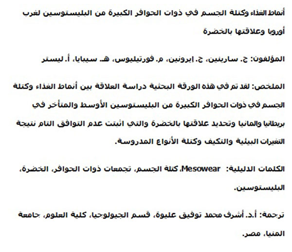
Translator: Ashraf M.T. Elewa
-
-
-
Review: The Princeton Field Guide to Mesozoic Sea Reptiles
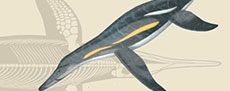 The Princeton Field Guide to Mesozoic Sea Reptiles
Article number: 26.1.1R
April 2023
 Poster Winners 2024