Lithification and biodiversity

The effects of lithification on fossil assemblage biodiversity and composition: An experimental test

Gwen M. Daley and Andrew M. Bush

Article number: 23(3):a53
https://doi.org/10.26879/1119
Copyright Paleontological Society, November 2020

Author biographies
Plain-language and multi-lingual abstracts
PDF version

Submission:  17 August 2020. Acceptance: 3 November 2020.

ABSTRACT

Lithification of unconsolidated sediment into solid rock can bias the tabulation of taxonomic diversity from fossil assemblages in several ways. Methodological biases result from the relative difficulty of extracting fossils from lithified sediments, whereas diagenetic biases result from poor preservation or destruction of fossils by dissolution or other processes. Here, we use an experimental approach to isolate the effects of methodological biases. Replicate samples of Pleistocene mollusks were collected from the same series of horizons at the same outcrop. One set of replicates was sieved and the other was cemented into artificial rocks before identifying and counting species. These procedures probably represent a best-case scenario for recovering biological signals: the artificial rocks were only poorly lithified, the sampling process was not highly destructive, and the smallest mollusks (< 4 mm) were excluded. However, minor biases were still introduced by the non-random nature of locating and identifying species in the lithified samples, despite efforts at random sampling. After standardizing sampling effort, the cemented samples actually appeared slightly more diverse than the uncemented replicates due to the oversampling of rare species. Assemblage composition was affected slightly by lithification, notably in the undersampling of oysters, whose irregular shells were probably more difficult to identify in matrix. The methodological effects of lithification doubtlessly vary - sample processing will be more destructive for some rocks and fossils - but methodological biases can be quite mild in some cases.

Gwen M. Daley. Department of Chemistry, Physics and Geology, Winthrop University, Rock Hill, South Carolina 29733, USA. daleyg@winthrop.edu
Andrew M. Bush. Department of Geosciences and Department of Ecology and Evolutionary Biology, University of Connecticut, 354 Mansfield Rd, Storrs, Connecticut 06269-1045, USA. andrew.bush@uconn.edu

Keywords: taphonomic bias; species richness; aragonite dissolution; Mollusca; paleoecology; Pleistocene

Daley, Gwen M. and Bush, Andrew M. 2020. The effects of lithification on fossil assemblage biodiversity and composition: An experimental test. Palaeontologia Electronica, 23(3):a53. https://doi.org/10.26879/1119
palaeo-electronica.org/content/2020/3204-lithification-and-biodiversity

Copyright: November 2020 Paleontological Society.
This is an open access article distributed under the terms of Attribution-NonCommercial-ShareAlike 4.0 International (CC BY-NC-SA 4.0), which permits users to copy and redistribute the material in any medium or format, provided it is not used for commercial purposes and the original author and source are credited, with indications if any changes are made.
creativecommons.org/licenses/by-nc-sa/4.0/

INTRODUCTION

Understanding the processes that generate and eliminate biodiversity is a central focus in both biology and paleobiology. However, paleobiologists face unique challenges in accurately estimating biodiversity because the formation and sampling of the fossil record can introduce biases not encountered in studies of the living biota. Here, we examine some of the potential biasing effects of lithification, the transformation of unconsolidated sediment into solid rock. Some effects of lithification (methodological biases) occur because fossils are prepared or extracted from lithified sediments using different techniques than those applied to unlithified sediments (Kowalewski et al., 2006; Nawrot, 2012). Many lithified fossil assemblages require time-consuming preparation by mechanical processes like hammering and scraping, leading to smaller sample sizes and fewer observed species. In contrast, unlithified sediments can frequently be wet-washed through sieves with no chemical treatment, and highly fossiliferous formations can yield hundreds to thousands of fossil specimens per kilogram of sediment with relatively little effort.

Variation in sample size can be counteracted by analytical standardization (e.g., Sanders, 1968; Hurlbert, 1971; Powell and Kowalewski, 2002; Kowalewski et al., 2006; Bush and Bambach, 2004; Chao and Jost, 2012), but sampling-standardization will not fix other methodological biases introduced by lithification (e.g., Hendy, 2009, 2010; Sessa et al., 2009). For example, sieved fossils can be manipulated and examined from all angles, making identification easier, whereas many fossils from lithified sediments cannot be removed from the rock matrix. It may be more difficult to locate small specimens in lithified samples, which could reduce their contribution to observed diversity, although small size classes are sometimes deliberately excluded from sieved unconsolidated material as well. In addition, the more intensive preparation methods applied to solid rocks could damage fossils (Kowalewski et al., 2006; Hendy, 2009; Nawrot, 2012). Silicified assemblages dissolved out of limestone can be more comparable to unlithified assemblages, although the silicification process itself can introduce other biases (e.g., Clapham, 2015; Pruss et al., 2015).

Lithification can also occur in conjunction with diagenetic biases introduced by poor preservation of some or all fossils due to compaction, dissolution, or other processes. In particular, aragonitic shells and skeletons dissolve more readily than those built of calcite or other minerals, which can lead to the underrepresentation or loss of common taxa like scleractinian corals and many mollusks (e.g., Koch and Sohl, 1983; Cherns and Wright, 2000, 2009; Cherns et al., 2008; Foote et al, 2015; Sanders et al., 2015). Fossil dissolution need not be directly linked with lithification (e.g., Nawrot, 2012; Sanders et al., 2015), although dissolution sometimes provides a source of cement (Cherns et al., 2008), in which case the two processes are connected. Just as small fossils may be harder to sample in lithified sediments, they may be particularly vulnerable to diagenetic loss (Cooper et al., 2006; Sessa et al., 2009; Sanders et al. 2015). Aragonite dissolution can impair the measurement of sample-level diversity (Koch and Sohl, 1983), but regional and global analyses of biodiversity appear to be more robust (Kidwell, 2005), probably due to patchy preservation of aragonitic taxa, often as molds (Bush and Bambach, 2004; Cherns et al., 2008; Dean et al., 2019).

It is critical to understand the strength of both methodological biases and diagenetic biases, as well as how each varies among geological contexts. For example, if methodological biases are strong and diagenetic biases are weak then additional sample preparation and/or modified preparation techniques might improve diversity estimates by revealing additional species. However, if diagenetic biases are strong and some fossil taxa are truly lost from the assemblage, then additional preparation of existing samples might not be fruitful. Instead, one’s time might be better spent searching for new samples on which diagenesis had less impact. As another example, consider a comparison of the rarefied species richness of bivalves from unlithified Cenozoic sediments to that of brachiopods from lithified Paleozoic rocks. If methodological biases are strong, then the comparison will be compromised by undercounting of diversity in the Paleozoic samples. However, if methodological biases are weak, then the comparison could be legitimate, because the preferential dissolution of aragonite is not an issue when all fossils are calcitic or phosphatic.

Most previous tests of the effects of lithification on fossil content were based on comparisons of unlithified and lithified samples from the same geological context that contained generally similar fauna. In some cases, the samples came from a narrow stratigraphic interval at a single outcrop where cementation was patchy (Nawrot, 2012; Sanders et al., 2015), whereas others included a broader range of samples (Hendy, 2009, 2010; Sessa et al., 2009). Several general patterns are evident from these studies, which all focused on Cretaceous and Cenozoic assemblages. First, lithification accompanied by aragonite dissolution significantly reduces apparent biodiversity, particularly in small size classes (< 5 mm or so). Some authors reported that biases were more severe for fully lithified sediments than for “poorly lithified” sediments, for which some disaggregation is possible with effort (Hendy, 2009). However, when lithification was not accompanied by aragonite dissolution, the effects on sample-level diversity were relatively mild, although, again, fossils less than 5 mm is size were under-represented (Nawrot, 2012; Sanders et al., 2015). For example, in a study of a patchily lithified Eocene shell bed, Sanders et al. (2015, table 1) found that rarefied species richness of lithified samples was 15 to 18, versus 17 to 19 for unlithified samples.

These studies suggest that methodological biases, in the absence of diagenetic biases, may not have a large effect on biodiversity tabulation. Taking another approach to the same problem, Hawkins et al. (2018) isolated the effects of methodological biases through computer simulation. After randomly placing virtual fossils within a prescribed space (the virtual rock), they passed planes through the space (i.e., sliced the rock) at different orientations and counted any fossil intersected by the plane. Rarefied species richness was 5-23% lower in the sliced, “lithified” samples relative to random draws of individuals from the original population, equivalent to a sieved sample. The “lithified” samples had lower evenness and higher mean size.

Here, we further test the effects of methodological biases associated with lithification using an experimental approach. We took replicate bulk samples of unconsolidated sediment from two highly fossiliferous Pleistocene formations from Florida (the Fort Thompson and Bermont), sieving one set of samples and counting all molluscan taxa following typical procedures for unlithified bulk samples (Daley et al., 2007). We then artificially cemented a subset of the replicate samples using hydraulic cement and tabulated diversity from these artificial rocks. Our treatments did not chemically or physically alter the sediment or fossils, and we therefore isolated the methodological effects of lithification from diagenetic effects like the dissolution of aragonitic shells (cf. Nawrot, 2012; Sanders et al., 2015; Hawkins et al., 2018). We examine the effects of lithification on both species richness and species composition.

MATERIALS AND METHODS

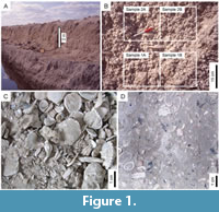Samples were collected from the Bermont and Fort Thompson formations at Caloosa Shell Quarry, Ruskin, Florida (Portell et al., 1995; Daley, 2001; Bush et al. 2002; Daley et al., 2007) (Figure 1A, B). These formations consisted of coarse shelly material with very fine quartz sand and a small amount of mud (Figure 1C). There was no significant natural cementation or evidence of diagenetic alteration such as recrystallization of aragonite.

The quarry wall was sampled at 30-cm increments using a shovel and pick. At each vertical position, replicate samples were taken directly adjacent to each other (Figure 1B). Each sample is referenced by a formation abbreviation (Ber or Ftt), a number that indicates vertical position, and a letter that distinguishes replicates (A or B). As part of previous paleoecological studies, one replicate from each set was sieved, and all mollusks retained on a 4-mm sieve were examined and identified (Daley, 2001; Daley et al. 2007). Taphonomic research indicates that death assemblages of these larger shells generally reflect the long-term composition of the adult living assemblage, whereas smaller shells are more affected by pre-burial processes like current sorting and by fluctuations in juvenile settlement (e.g., Cummins et al., 1986; Kidwell, 2001, 2002; Nawrot, 2012). To avoid double-counting, shells were counted following the procedures outlined by Daley (2001). For example, bivalve specimens were only counted if they included enough of the hinge to allow species-level identification, and the number of bivalve specimens for each species was divided by two to account for each bivalve shell having two valves (e.g., Bambach and Kowalewski, 2000; Kowalewski and Hoffmeister, 2003).

Artificial Cementation

Three replicate samples from each formation were cemented using Sakrete^TM bolt and rail cement anchor. This product was designed to anchor bolts in concrete slabs, and thus was engineered to flow into tight spaces, like those between shells. The fine-grained cementing mixture filled in most of the visible void spaces within the body of the unconsolidated sediment, creating a fair simulacrum of a real rock. One kilogram of dry unconsolidated sediment sample was gently mixed by hand with 250 grams of dry cementing agent, ensuring that the dry cement was evenly distributed throughout the sediment. Five hundred mL of water was then poured into the sample and mixed by hand. The wet, pliable mixture was transferred to a 36×8 cm mold, where it was allowed to set undisturbed for an hour, at which time it was sufficiently rigid to transfer from the mold. To allow ample time for the cementation reactions to run to completion, the newly formed rock tiles were allowed to sit for at least five days out of direct sunlight.

The cement adhered both to the quartz sand and the shelly material, resulting in samples of artificially cemented, highly fossiliferous, argillaceous sandstone (Figure 1D). The degree of cementation was sufficient that fossils could be removed using tools with some effort. Similar to Nawrot’s (2012) assemblages, these samples could be described as “poorly lithified.”

Natural rocks vary in degree of cementation, and methods for extracting and counting fossils from lithified rocks vary as well. Thus, no single experimental protocol can perfectly replicate all situations. Our approach represents one reasonable scenario and replicates the contrast between sieving an assemblage on one hand and finding and preparing fossils from a cemented matrix on the other. However, as we address in the Discussion, the exact effects of lithification certainly depend to some extent on rock type, fossil type, and preparation methods.

Data Collection

The rock matrix was slowly removed to reveal the fossils using dental picks and soft nylon brushes. Larger hand tools, wire brushes, chisels, and mechanical devices like air abrasive units and drills were not used. The samples were not washed during processing nor was sediment removed from the rock sieved for small fossils.

To keep the experimental and control data comparable, we used the same rules for recognizing a countable bivalve or gastropod specimen that were used by Daley (2001) and Daley et al. (2007) for the unlithified replicates. For bivalves, the presence of the hinge structure had to be confirmed by excavating enough of the matrix and/or overlying shell material to see that the structure was present. Similar excavations were necessary for gastropods. It was not necessary to remove the specimen from the rock tile matrix to count it as a specimen. Given that the unconsolidated samples were processed on a 4 mm sieve, only specimens that were at least 4 mm in at least one dimension were counted from the experimental samples. Any specimen that was less than 1 mm long in any dimension was not counted. The exclusion of small specimens was required for consistency with the previously collected data. In addition, however, all previous studies agree that fossils smaller than several millimeters are under-represented in lithified assemblages (e.g., Nawrot, 2012; Sanders et al., 2015), so excluding them allows us to concentrate on the fate of the larger size classes.

Each rock slab was examined using a 4x magnifying lamp, starting with the upper left-hand corner. Any shells protruding from the body of the tile were further examined and excavated if there was a chance the shell was a countable fragment as defined above. A combination of picking with the dental picks and vigorous brushing with a nylon brush was a slow but effective method of excavation. Specimens that came loose from the rock tile were given an identification number, identified to the species level, and placed in a bag. If the specimen could be identified without removing it from the rock tile, it was given an identification number and left in place. If it later became necessary to remove the specimen, it would be transferred to the same bag as the other members of its species.

As specimens became harder to find, the tops and sides of the rock were brushed and scraped, exposing more shells. Collection continued until 100 specimens had been identified or a maximum of 10 hours of processing had been completed. The number of bivalve hinge fragments counted for each species was divided by two and the fractions rounded up to account for each bivalve having two valves to its shell (Bambach and Kowalewski, 2000; Kowalewski and Hoffmeister, 2003). The raw data set is provided in the Appendix.

Data Analysis

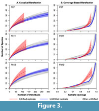
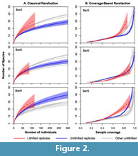Sampling intensity was standardized using classical rarefaction (Sanders, 1968; Hurlbert, 1971) and coverage-based rarefaction (Chao and Jost, 2012), which is similar to Alroy’s (2010 a,b) shareholder quorum subsampling method. The rarefaction analyses were conducted using the iNEXT function in the iNEXT package (Hsieh et al., 2016) in the R programming environment (R Core Team, 2017). This function both conducts rarefaction (reducing sampling intensity below the observed value) and extrapolation (predicting diversity at higher sampling intensity than observed). We focus on the rarefaction results, but include the extrapolation results in Figure 2 and Figure 3 (dashed lines). Shannon-Wiener diversity (H) and evenness (exp[H]/S) were determined using PAST software package (Hammer et al., 2001). To examine differences in the abundance structure of the lithified and unlithified samples, rank abundance plots were created using the rank abundance function in the BiodiversityR package in R (Kindt and Coe, 2005).

Given that lithification is generally presumed to suppress the abundance and diversity of small-bodied species, we also examined the effects of lithification on body-size distribution of sampled specimens (bearing in mind that specimens < 4 mm, which are most vulnerable to this bias, were not included in the study). We categorized all species into three size categories based on maximum dimension following Daley (2017): small (4-15 mm), medium (15-50 mm), and large (> 50 mm). These assignments were based on measurements of a subset of specimens. Although this analysis will not capture subtle changes in the body-size distribution, it should detect large, obvious effects. Confidence intervals on proportions were calculated using Wilson’s method (Brown et al., 2001).

Variation in species composition was visualized using principal coordinates analysis based on Bray-Curtis dissimilarity (e.g., Tyler and Kowalewski, 2014). Species abundances were standardized to proportions due to the great differences in sample size between the lithified and unlithified samples. Methods like detrended correspondence analysis and non-metric multidimensional scaling are often preferred because they can counteract the “arch” or “horseshoe” effect (e.g., Holland et al., 2001; Bush and Brame, 2010). However, this effect is observed when samples vary considerably in species composition, and the Fort Thompson and Bermont samples contain the same set of species. For example, the only species that did not occur in both formations were ones whose average sample-level abundance was less than 0.2%.

RESULTS

Diversity

Given the slower pace of data collection, the sample sizes of the experimentally cemented samples were much smaller than those of the unconsolidated control samples (Table 1, Table 2). It took approximately 10 hours to find 40-50 countable individuals from the cemented samples after the bivalve material had been halved (4-5 individuals/hour). In contrast, the unconsolidated samples of the same material required approximately three hours to yield 400-650 countable individuals (133-217 individuals/hour). As a result, the raw number of species recovered was lower for the lithified samples.

However, the cemented samples had slightly higher species richness than their unconsolidated replicates when the latter were rarefied to match the sampling intensity of the former, although the difference was not always significant (Figure 2, Figure 3). With one exception (Ber6), the cemented samples also had higher species richness than all of the rarefied unconsolidated samples from the same formation. Results were similar for both rarefaction methods.

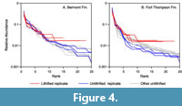For both formations, the rank abundance curves for the lithified samples generally overlapped those of the unlithified samples for the 10 most common species (i.e., rank ≤ 10; Figure 4). At higher ranks, the curves for the lithified samples flatten out, reflecting the presence of numerous species represented by a single specimen (the lithified samples contained between 43 and 62 specimens, so calculated proportional abundances for singleton species range from 2.3% to 1.6%). In contrast, the curves for the unlithified samples continued to decline. A randomization test suggests that the number of singleton species in the lithified replicates is in fact unexpectedly high. We subsampled each unlithified replicate down to the sample size of the corresponding lithified sample 10,000 times, tabulating the number of singletons for each iteration. The number of singletons in the lithified samples always fell in the upper ends of these distributions, with percentiles of 99.6, 96.8, 97.4, 99.8, 71.5, and 85.0 for Ftt7, Ftt11, Ftt12, Ber5, Ber6, and Ber9, respectively. The number of singletons in the lithified samples is statistically significantly higher than expected for some samples (percentile > 95.0 for individual single-sided tests with α = 0.05, or > 99.2 with a Bonferroni correction), and the fact that all percentiles are high indicates an overall tendency towards increased singletons.

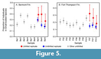The cemented samples also had significantly higher evenness than the unconsolidated samples from the same formation (Table 1, Table 2), and the proportion of specimens belonging to small-bodied species (4-15 mm) was slightly higher in each cemented sample than in the corresponding unconsolidated replicate (Figure 5).

Species Composition

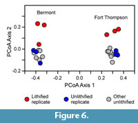The first principal coordinate axis separated the samples from the Fort Thompson Formation from those from the Bermont (Figure 6), reflecting the different composition of the two faunas, which can be seen more directly in the relative abundance data for the 10 most abundant species (Figure 7). For each formation, the second principal coordinate axis separated the unlithified samples from the lithified ones, suggesting a consistent change in composition caused by lithification. For the Fort Thompson samples, the lithified and unlithified samples are separated by a clear gap (Figure 6). One of the lithified Bermont samples plots closer to the cluster of unlithified samples (lowermost red circle, representing sample Ber9A). However, the unlithified replicate of this sample, Ber9B, is represented by the most negative blue circle in the cluster, so Ber9A is in fact shifted in a positive direction from its direct replicate, consistent with the direction of displacement for the other lithified samples.

DISCUSSION

In some cases, mechanical preparation of fossils from lithified sediments may destroy fossils, particularly delicate ones, and preferential destruction of certain species could affect studies of diversity and assemblage composition. However, fossil destruction was not an important bias in our poorly lithified samples. Instead, minor biases likely stemmed from changes in the probability that a particular species was noticed, identified, and counted during data collection.

With sieved samples, one can systematically examine all specimens, viewing each in three dimensions for identifying characteristics. Whole fossils can be separated from unidentifiable fragments, and each species can be placed in a separate tray or container. In the case of our sieved samples, we counted all bivalve and gastropod specimens that met certain criteria of size and completeness. However, in a lithified sample, it is more challenging to count every specimen due to the increased difficulty of fossil extraction. The paleontologist’s ability to notice and identify a specimen imposes another filter: certain types of specimens are more likely to be noticed and/or more likely to be identifiable when entombed in matrix. Both species richness and species composition were affected by this perceptual filter, albeit in different ways.

Species Richness and Rarity

Surprisingly, the experimentally cemented samples tended to have slightly higher species richness after sampling standardization than did their unconsolidated replicates (Figure 2, Figure 3). Given that pairs of replicates were drawn from the same sampling distribution, the differences in diversity must reflect differences in how fossils were identified and counted.

The rank abundance plots show that rare species were oversampled in the lithified samples relative to the unlithified ones - had sampling been random in the lithified samples, then their rank abundance curves would overlap the others (Figure 4). Instead, the lithified samples generally include an unusual number of single-individual species. Oversampling of rare species explains the elevated standardized diversity (Figure 2, Figure 3) and evenness (Table 1, Table 2). We attribute this oversampling to the natural human tendency to notice the unusual and overlook the mundane. For sieved bulk samples, it is much easier to override this instinct.

Previous studies indicated that lithification combined with aragonite dissolution notably suppressed the apparent diversity of molluscan fossil assemblages (e.g., Sessa et al., 2009; Hendy, 2009). However, other studies have indicated that the methodological effects of lithification on diversity tabulation (the effects related to sample preparation and not diagenesis) were fairly mild for macrofossils greater than a few millimeters in size, once sample sizes were standardized by rarefaction (e.g., Nawrot, 2012; Sanders et al., 2015). Our results indicate that, somewhat surprisingly, lithification can even be associated with slightly higher observed diversity.

Species Composition

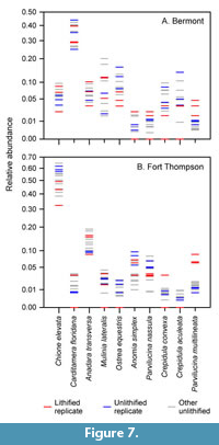
Species richness is highly sensitive to the presence of rare species, but the results of the principal coordinates analyses largely reflect variation in the relative abundances of common species, particularly considering that we did not log-transform species abundances. Despite containing the same set of species, the faunas of the two formations are easily distinguishable based on relative abundance, and lithification did not obscure these basic patterns (Figure 6, Figure 7).

The lithified samples are all displaced in a positive direction on principal component axis two (Figure 6), suggesting that lithification affected faunal composition in similar ways in both sets of samples. However, lithification did not clearly alter the apparent relative abundance of many species, and others were affected differently in the two faunas (Figure 7). For example, Chione elevata has lower relative abundance in the lithified samples (red) than in the unlithified replicates (blue) in the Fort Thompson, but not in the Bermont.

There are, however, a few consistent differences in species’ relative abundances between the lithified and unlithified samples. Most notably, Ostrea equestris, the fifth most abundant species in the dataset, is under-represented in the lithified samples relative to the unlithified replicates in both data sets (Figure 7). Ostrea shells are irregular and may have been harder to distinguish from shell fragments when embedded in matrix, which could lead to undercounting - a reverse of the “Chlamys effect,” which describes the over-counting of easily identified species (Kowalewski et al., 2003). Parvilucina multilineata, the tenth most abundant species overall, is over-represented in the lithified samples, although it is unclear to us why this might be, other than, perhaps, random chance. Crepidula aculeata, the ninth most abundant species, is under-represented in the lithified samples, but the congeneric Crepidula convexa is not under-represented as consistently, so the pattern for this morphotype is not entirely clear.

Given the common assumption that lithification preferentially obscures small fossils, it is somewhat surprising that individuals belonging to small-bodied species were slightly over-represented in the cemented samples (Figure 5). However, specimens less than 4 mm in size were completely excluded from the analysis, and previous literature suggests that the size-bias would primarily affect this size class (e.g., Cooper et al., 2006; Sessa et al., 2009). In other words, once shells smaller than a few millimeters were excluded, the size-bias was not particularly important (also see, for example, Nawrot, 2012).

In sum, lithification had relatively mild effects on the apparent species composition of these samples. The faunas of the two formations, which contained heavily overlapping sets of species, could still be distinguished. Lithification might have depressed the apparent relative abundance of the oyster Ostrea equestris, possibly because it is irregular in morphology and less easy to distinguish as a countable specimen when ensconced in matrix. Further studies would be needed to confirm this effect.

Effects of Lithification and Diagenesis on Diversity: General Models

I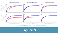n Figure 8, we illustrate some of the ways that lithification and diagenesis could alter the apparent diversity of a sample of shelly fossils using classical rarefaction curves. The blue rarefaction curves represent bulk samples from pristine, unaltered assemblages, from which specimens were tabulated comprehensively (every specimen tabulated) or at random. The red rarefaction curves represent assemblages affected by lithification or some other diagenetic process. The total species richness of a sample is represented by the rarefaction curve’s asymptote, and evenness is represented by the initial slope (e.g., Olszewski, 2004). In general, fewer individuals will be counted from lithified samples due to the increased difficulty of data collection, but we show the same maximum samples size for all rarefaction curves for the sake of comparison.

In Figure 8A-C, no species were lost due to diagenesis or sample processing, such that the blue and red rarefaction curves asymptote at the same value given high enough sampling intensity. In Figure 8B, lithification did not alter the relative abundance distribution of the assemblage, such that the rarefaction curves coincide. However, in Figure 8A, C, the apparent relative abundances of species in the lithified sample were altered by either diagenetic or methodological effects. In Figure 8C, rare species were preferentially sampled from the altered sample, increasing the apparent species richness at low sampling levels. This preferential sampling could occur due to collector bias, as in the present study, or if common species were poorly preserved or difficult to recognize due to small size, partial dissolution, irregular morphology, etc. In Figure 8A, common species were oversampled in the diagenetically altered sample, lowering its apparent species richness at low sampling levels. In cases like these (Figure 8A, C), additional collecting should improve the diversity estimate (i.e., rarefaction curves should begin to converge) because no species were entirely lost.

In Figure 8D-F, some species were lost entirely due to aragonite dissolution, preferential destruction of fragile species during processing, or some other process. No amount of extra sampling would recover these species, which is indicated graphically by the red and blue rarefaction curves rising to different asymptotes. If rare species are preferentially lost, the affected sample will be less even and have fewer species than the pristine sample at all sampling intensities (Figure 8D). However, if common species are preferentially lost, the remaining rare species will be sampled more quickly, and species richness can appear higher at low sampling intensity before asymptoting at a lower value (Figure 8F).

Other Rock Types

When lithification is accompanied by aragonite dissolution (Sessa et al., 2009; Hendy, 2009), the effects on diversity can be large, corresponding to Figure 8D-F (i.e., decrease in observable species richness). In the absence of preferential destruction of certain fossil species by diagenesis or preparation, the effects of lithification are relatively limited for larger fossils (Nawrot, 2012; Sanders et al., 2015), reflecting changes in the observed relative abundance distribution rather than loss of species (Figure 8A-C). However, it is worth emphasizing that our cemented samples were equivalent to “poorly lithified” sediments, and the methodological effects of lithification may differ for more completely cemented rocks prepared with other methods. It is also worth emphasizing that studies of the effects of lithification on biodiversity have focused on late Mesozoic to Cenozoic molluscan shell beds (e.g., Sessa et al., 2009; Hendy, 2009; Nawrot, 2012; Sanders et al., 2015), although aragonite dissolution has been discussed more broadly (e.g., Cherns and Wright, 2000, 2009; Cherns et al., 2008; Hsieh et al., 2019).

What about Paleozoic and older Mesozoic rocks, which are often more completely cemented? The exact effects of lithification probably depend on how the fossils are distributed through the rock, the physical properties of the rock, the mode of fossil preservation, and the preparation and sampling methods. For example, many Paleozoic fossil assemblages are preserved in thin shell beds or on bedding planes (Kidwell and Brenchley, 1994), and these assemblages can be exquisitely exposed if lithified limestone or sandstone beds are separated by easily eroded mud. This style of preservation is common, for example, in the Ordovician of the Cincinnati, Ohio, region, which has served as the basis for many paleobiological studies (e.g., Holland et al., 2001). The methodological effects of lithification are probably minimized in these assemblages; fossils that are more than a couple millimeters in size can be readily observed, and a comprehensive census of a bedding plane can reduce human-induced non-randomness. Also, destructive preparation in not needed. A study restricted to brachiopods might suffer little bias, corresponding perhaps with Figure 8B. However, a whole-fauna analysis might correspond instead with Figure 8E due to diagenetic loss of mollusks.

The methodological biases of lithification may be most severe for carbonate fossils ensconced within well-cemented limestones, in which case extraction can be quite difficult. Fossils in well-cemented siliciclastic rocks can be easier to find due to the contrast in composition between rock and fossil - when prepared using hammers, chisels, and rock splitters, cemented sandstones will tend to fracture along planes of weakness, which are often created by fossil shells or their molds. If fossils are concentrated along a particular horizon, that horizon will be exposed, providing an assemblage somewhat like a naturally exposed bedding-plane assemblage.

If fossils are distributed more randomly in a well-cemented rock, or in a thicker shell bed, they can be found by breaking a sample into smaller and smaller pieces. It is possible that small fossils may be somewhat under-sampled during this type of processing because large fossils create larger areas of weakness within a rock. However, under-sampling of small fossils will be reduced by more complete processing of a sample (i.e., breaking it into more and smaller pieces). However, this processing could reduce large fossils to unidentifiable or uncountable fragments, even as it exposes complete small fossils on fracture faces. Thus, the extent of bias depends on the choices made during sample preparation. Also, size-related bias will only occur if large and small fossils co-occur in the same sample; if all fossils are similar in size, then size will not affect the probability of collection. In our experience with Paleozoic fossils (e.g., Bush et al. 2015), fossils that are 4-5 mm or larger are relatively easy to find, although fine morphological details may not be preserved in molds in coarser sediments. Again, if diagenetic processes or sample preparation have eliminated some taxa, then the complete diversity of a sample cannot be recovered (Figure 8D-F). In other cases, however, methodological biases could have a range of effects (Figure 8A-C), depending on how they affect the relative abundance distribution.

In our poorly lithified samples, we had some capacity to remove sediment from shell surfaces, which may have mitigated perceptual biases to some extent by improving our ability to identify all species. The under-counting of certain taxa might be more severe in well-cemented samples where sediment cannot be removed easily from fossils. Moldic preservation may alleviate this problem, however, if the impressions of shell surfaces are well preserved.

In sum, the effects of lithification on biological patterns are probably highly variable, and for some studies, methodological biases are probably minor. Even when lithification imparts more serious biases, these biases may not be an impediment if all samples in a study are biased similarly. Given that lithification and fossil dissolution can be linked, lithification may provide a useful warning that diagenetic biases should be carefully evaluated, even if the methodological effects of lithification are not the primary source of bias.

CONCLUSIONS

Lithification can affect the measurement of species richness both through methodological biases related to the sampling of solid rock and through diagenetic biases related to the alteration and/or destruction of fossils by dissolution and other processes. To isolate the effects of methodological biases, we cemented samples of unconsolidated, fossiliferous Pleistocene sediment into artificial rocks. We compared the observed biodiversity of these samples to that measured from replicate control samples that were not cemented and that were sieved. The comparison focuses specifically on the biases introduced by changing the physical nature of the matrix surrounding the fossils without altering or destroying any fossils.

Our sampling of the poorly lithified artificial rocks was not destructive to the fossils, and we excluded fossils smaller than 4 mm, so this test probably represents a best-case scenario for recovering biological patterns. Even so, mild biases were introduced by non-randomness in locating and identifying specimens in the lithified samples. The lithified samples had slightly higher sampling-standardized species richness than the unlithified control samples due to over-representation of rare species, which we ascribe to the human tendency to notice new and rare items and overlook common items.

The effects of lithification on assemblage composition were similarly mild. Lithification did not obscure the differences in species relative abundance between samples from two different formations, such that these two faunas were still distinguishable. However, the oyster Ostrea equestris was under-represented in all lithified samples, perhaps because its irregular morphology was difficult to identify when obscured by matrix.

Several studies have now shown that lithification has only mild effects on the observed diversity and composition of fossil assemblages, at least when sampling intensity is standardized, very small fossils are excluded, fossils can be exposed for examination without the preferential destruction of some species, and diagenetic destruction is not an issue. In real rocks, the effects of lithification on biological patterns will vary considerably and should be evaluated on a case-by-case basis.

ACKNOWLEDGMENTS

Our thanks to two anonymous reviewers for helpful comments on the manuscript.

REFERENCES

Alroy, J. 2010a. Fair sampling of taxonomic richness and unbiased estimation of origination and extinction rates, p. 55-80. In Alroy, J. and Hunt, G. (eds.), Quantitative Methods in Paleobiology. Paleontological Society Papers, 16. https://doi.org/10.1017/s1089332600001819

Alroy, J. 2010b. Geographical, environmental and intrinsic biotic controls on Phanerozoic marine diversification. Palaeontology, 53:1211-1235. https://doi.org/10.1111/j.1475-4983.2010.01011.x

Bambach, R.K. and Kowalewski, M. 2000. How to count fossils. Geological Society of America Abstracts with Programs, 32(7):332.

Brown, L.D., Cai, T.T., and DasGupta, A. 2001. Interval estimation for a binomial proportion. Statistical Science, 16:101-133. https://doi.org/10.1214/ss/1009213286

Bush, A.M. and Bambach, R.K. 2004. Did alpha diversity increase through the Phanerozoic? Lifting the veils of taphonomic, latitudinal, and environmental biases. Journal of Geology, 112:625-642. https://doi.org/10.1086/424576

Bush, A. M. and Brame, R.I. 2010. Multiple paleoecological controls on the composition of marine fossil assemblages from the Frasnian (Late Devonian) of Virginia, with a comparison of ordination methods. Paleobiology, 36:573-591. https://doi.org/10.1666/07022.1

Bush, A.M., Csonka, J.D., DiRenzo, G.V., Over, D.J., and Beard, J.A. 2015. Revised correlation of the Frasnian-Famennian boundary and Kellwasser events (Upper Devonian) in shallow marine paleoenvironments of New York State. Palaeogeography, Palaeoclimatology, Palaeoecology, 433:233-246. https://doi.org/10.1016/j.palaeo.2015.05.009

Bush, A.M., Powell, M.G., Arnold, W.S., Bert, T.M., and Daley, G.M. 2002. Time-averaging, evolution, and morphologic variation. Paleobiology, 28:9-25. https://doi.org/10.1666/0094-8373(2002)028<0009:TAEAMV>2.0.CO;2

Chao, A. and Jost, L. 2012. Coverage-based rarefaction and extrapolation: Standardizing samples by completeness rather than size. Ecology, 93:2533-2547. https://doi.org/10.1890/11-1952.1

Cherns, L. and Wright, V.P. 2000. Missing molluscs as evidence of large-scale, early skeletal aragonite dissolution in a Silurian sea. Geology, 28:791-794. https://doi.org/10.1130/0091-7613(2000)28<791:MMAEOL>2.0.CO;2

Cherns, L. and Wright, V.P. 2009. Quantifying the impacts of early diagenetic aragonite dissolution on the fossil record. Palaios, 24:756-771. https://doi.org/10.2110/palo.2008.p08-134r

Cherns, L., Wheeley, J.R., and Wright, V.P. 2008. Taphonomic windows and molluscan preservation. Palaeogeography, Palaeoclimatology, Palaeoecology, 270:220-229. https://doi.org/10.1016/j.palaeo.2008.07.012

Clapham, M.E. 2015. Ecological consequences of the Guadalupian extinction and its role in the brachiopod-mollusk transition. Paleobiology, 41:266-279. https://doi.org/10.1017/pab.2014.15

Cooper, R.A., Maxwell, P.A., Crampton, J.S., Beu, A.G., Jones, C.M., and Marshall, B.A. 2006. Completeness of the fossil record: Estimating losses due to small body size. Geology, 34:241-244. https://doi.org/10.1130/G22206.1

Cummins, H., Powell, E.N., Stanton, R.J., and Staff, G. 1986. The size-frequency distribution in palaeoecology: Effects of taphonomic processes during formation of molluscan death assemblages in Texas bays. Palaeontology, 29: 495-518.

Daley, G.M. 2001. Creating a paleoecological framework for evolutionary and paleoecological studies: An example from the Fort Thompson Formation (Pleistocene) of Florida. Palaios, 17:419-434. https://doi.org/10.1669/0883-1351(2002)017<0419:capffe>2.0.co;2

Daley, G.M., Ostrowski, S., and Geary, D.H. 2007. Paleoenvironmentally correlated differences in a classic predator-prey system: the bivalve Chione elevata and its gastropod predators. Palaios, 22:166-173. https://doi.org/10.2110/palo.2005.p05-057r

Daley, G.M. 2017. Diversity and faunal composition in fragments. Palaios, 32:639-646. https://doi.org/10.2110/palo.2016.101

Dean, C.D., Allison, P.A., Hampson, G.J., and Hill, J. 2019. Aragonite bias exhibits systematic spatial variation in the late Cretaceous Western Interior Seaway, North America. Paleobiology, 45:571-597. https://doi.org/10.1017/pab.2019.33

Foote, M., Crampton, J.S., Beu, A.G., and Nelson, C.S. 2015. Aragonite bias and lack of bias, in the fossil record: lithological, environmental, and ecological controls. Paleobiology, 41:245-265. https://doi.org/10.1017/pab.2014.16

Hammer, Ø., Harper, D.A.T., and Ryan, P.D. 2001. PAST: Paleontological statistics software package for education and data analysis. Palaeontologia Electronica, 4.1.1:1-9. http://palaeo-electronica.org/2001_1/past/issue1_01.htm

Hawkins, A.D., Kowalewski, M., and Xiao, S. 2018. Breaking down the lithification bias: the effect of preferential sampling of larger specimens on the estimate of species richness, evenness, and average specimen size. Paleobiology, 44:326-345. https://doi.org/10.1017/pab.2017.39

Hendy, A.J.W. 2009. The influence on lithification on Cenozoic marine biodiversity trends. Paleobiology, 35:51-62. https://doi.org/10.1666/07047.1

Hendy, A.J.W. 2010. Taphonomic overprints on Phanerozoic trends in biodiversity: Lithification and other secular megabiases, p. 19-77. In Allison, P.A. and Bottjer, D.J. (eds.), Taphonomy. Topics in Geobiology, 32. Springer, Dordrecht. https://doi.org/10.1007/978-90-481-8643-3_2

Holland, S.M., Miller, A.I., Meyer, D.L., and Dattilo, B.F. 2001. The detection and importance of subtle biofacies within a single lithofacies: the Upper Ordovician Kope Formation of the Cincinnati, Ohio region. Palaios, 16:205-217. https://doi.org/10.2307/3515600

Hsieh, S., Bush, A.M., and Bennington, J.B. 2019. Were bivalves ecologically dominant over brachiopods in the late Paleozoic? A test using exceptionally preserved fossil assemblages. Paleobiology, 45:265-279. https://doi.org/10.1017/pab.2019.3

Hsieh, T.C., Ma, K.H., and Chao, A. 2016. iNEXT: An R package for interpolation and extrapolation of species diversity (Hill numbers). Methods in Ecology and Evolution, 7:1451-1456. https://doi.org/10.1111/2041-210x.12613

Hurlbert, S.H. 1971. The nonconcept of species diversity: a critique and alternative parameters. Ecology, 52:577-586. https://doi.org/10.2307/1934145

Kidwell, S.M. 2001. Preservation of species abundance in marine death assemblages. Science, 294:1091-1094. https://doi.org/10.1126/science.1064539

Kidwell, S.M. 2002. Mesh-size effects on the ecological fidelity of death assemblages: A meta-analysis of molluscan live-dead studies. Geobios, 35:107-119. https://doi.org/10.1016/s0016-6995(02)00052-9

Kidwell, S.M. 2005. Shell composition has no net impact on large-scale evolutionary patterns in mollusks. Science, 307:914-917. https://doi.org/10.1126/science.1106654

Kidwell, S.M. and Brenchley, P.J. 1994. Patterns in bioclastic accumulation through the Phanerozoic: changes in input or in destruction? Geology, 22:1139-1143. https://doi.org/10.1130/0091-7613(1994)022<1139:pibatt>2.3.co;2

Kindt, R. and Coe, R. 2005. Tree diversity analysis: a manual and software for common statistical methods for ecological and biodiversity studies. World Agroforestry Centre, Nairobi, Kenya. http://www.worldagroforestry.org/output/tree-diversity-analysis

Koch, C.F. and Sohl, N.F. 1983. Preservational effects in paleoecological studies: Cretaceous mollusc examples. Paleobiology, 9:26-34. https://doi.org/10.1017/s0094837300007351

Kowalewski, M. and Hoffmeister, A.P. 2003. Sieves and fossils: Effects of mesh size on paleontological patterns. Palaios, 18:460-469. https://doi.org/10.1669/0883-1351(2003)018<0460:SAFEOM>2.0.CO;2

Kowalewski, M., Carroll, M., Casazza, L., Gupta, N.S., Hannisdal, B., Hendy, A., Richard. A., Jr, LaBarbera, M., Lazo, D.G., and Messina, C. 2003. Quantitative fidelity of brachiopod-mollusk assemblages from modern subtidal environments of San Juan Islands, USA. Journal of Taphonomy, 1:43-65.

Kowalewski, M., Kiessling, W., Aberhan, M., Fürsich, F.T., Scarponi, D., Barbour Wood, S.L., and Hoffmeister, A.P. 2006. Ecological, taxonomic, and taphonomic components of the post-Paleozoic increase in sample-level species diversity of marine benthos. Paleobiology, 32:533-561. https://doi.org/10.1666/05074.1

Nawrot, R. 2012. Decomposing lithification bias: Preservation of local diversity structure in recently cemented storm-beach carbonate sands, San Salvador, Bahamas. Palaios, 27:190-205. https://doi.org/10.2110/palo.2011.p11-028r

Olszewski, T.D. 2004. A unified mathematical framework for the measurement of richness and evenness within and among multiple communities. Oikos, 104:377-387. https://doi.org/10.1111/j.0030-1299.2004.12519.x

Portell, R.W., Schindler, K.S., and Nicol, D. 1995. Biostratigraphy and paleoecology of the Pleistocene invertebrates from the Leisey Shell Pits, Hillsborough County, Florida. Bulletin of the Florida Museum of Natural History, 37:127-164.

Powell, M.G. and Kowalewski, M. 2002. Increase in evenness and sampled alpha diversity through the Phanerozoic: Comparison of early Paleozoic and Cenozoic marine fossil assemblages. Geology, 30:331-334. https://doi.org/10.1130/0091-7613(2002)030<0331:iieasa>2.0.co;2

Pruss, S.B., Payne, J.L., and Westacott, S. 2015. Taphonomic bias of selective silicification revealed by paired petrographic and insoluble residue analysis. Palaios, 30:620-626. https://doi.org/10.2110/palo.2014.105

R Core Team. 2017. R: A Language and Environment for Statistical Computing. R Foundation for Statistical Computing, Vienna, Austria. https://www.R-project.org

Sanders, H.L. 1968. Marine benthic diversity: a comparative study. American Naturalist, 102:243-282. https://doi.org/10.1086/282541

Sanders, M.T., Merle, D., and Villier, L. 2015. The molluscs of the “Falunière” of Grignon (Middle Lutetian, Yvelines, France): Quantification of lithification bias and its impact on the biodiversity assessment of the Middle Eocene of Western Europe. Geodiversitas, 37:345-365. https://doi.org/10.5252/g2015n3a4

Sessa, J.A., Patzkowsky, M.E., and Bralower, T.J. 2009. The impact of lithification on the diversity, size distribution, and recovery dynamics of marine invertebrate assemblages. Geology, 37:115-118. https://doi.org/10.1130/g25286a.1

Tyler, C.L. and Kowalewski, M. 2014. The utility of marine benthic associations as a multivariate proxy for paleobathymetry. PLoS One, 9:e95711. https://doi.org/10.1371/journal.pone.0095711