CFD of ammonoid shells

Computational fluid dynamics modeling of fossil ammonoid shells

Nicholas Hebdon, Kathleen A. Ritterbush, and YunJi Choi

Article number: 23(1):a21
https://doi.org/10.26879/956
Copyright Paleontological Society, April 2020

Author biographies
Plain-language and multi-lingual abstracts
PDF version

Submission:  31 December 2019. Acceptance: 1 April 2020.

ABSTRACT

We use three-dimensional (3D) numerical models to examine critical hydrodynamic characteristics of a range of shell shapes found in extinct ammonoid cephalopods. Ammonoids are incredibly abundant in the fossil record and were likely a major component of ancient marine ecosystems. Despite their fossil abundance we lack significant soft body remains, which has made it historically difficult to investigate the potential life modes and ecological roles that these organisms played. By employing numerical tools to study how the morphology of a shell affected an ammonite’s hydrodynamics, we can build a foundation for hypothesizing and testing changes in the organism’s capabilities through time. To achieve this goal, the study was carried out in two major steps. First, we applied a number of simulation methods to a known problem, the drag coefficient of a half-sphere, to select the most appropriate modeling method that is accurate and efficient. These were further checked against previous experimental results on ammonoid hydrodynamics. Next, we produced 3D models of the ammonoid shells using Blender and Zbrush where each shell model emulated a specific fossil ammonoid, recent Nautilus, or an idealized shell forms created by systematically varying shell inflation and umbilical exposure. We test the hypothesis that both the overall shell inflation and umbilical exposure will increase the drag experienced by a similarly sized ammonoid shell as it moves through water relative to other morphologies. ANSYS FLUENT was employed to execute the study. We further compare our simulation results to published experimental measurements of drag on ammonoid fossil replicas and live Nautilus. The simulation results provide accuracy within an order of magnitude of published values, across the tested range of water flow velocities (1 - 50 cm/s). The simulated drag measurements demonstrate a first-order sensitivity to shell inflation, with a second-order effect from umbilical exposure. The impact of a larger umbilical exposure (shells that are more evolute) is minimal at low velocities, but substantial at higher velocities. We conclude that the overall shell inflation and umbilical exposure influence an individual shell’s drag coefficient, therefore, influence the hydrodynamic efficiency.

Nicholas Hebdon. University of Utah Department of Geology and Geophysics, Frederick Albert Sutton Building, 115 S 1460 E, Salt Lake City, Utah 84112, USA. nicholas.hebdon@utah.edu
Kathleen A. Ritterbush. University of Utah Department of Geology and Geophysics, Frederick Albert Sutton Building, 115 S 1460 E, Salt Lake City, Utah 84112, USA. k.ritterbush@utah.edu
YunJi Choi. Jacobs Engineering, yunji.choi@jacobs.com

Keywords: biomechanics; functional morphology; morphometrics; paleoecology; computer simulation; fluid dynamics

Final citation: Hebdon, Nicholas, Ritterbush, Kathleen A. and Choi, YunJi. 2020. Computational fluid dynamics modeling of fossil ammonoid shells. Palaeontologia Electronica, 23(1):a21. https://doi.org/10.26879/956
palaeo-electronica.org/content/2020/3003-cfd-of-ammonoid-shells

Copyright: April 2020 Paleontological Society.
This is an open access article distributed under the terms of Attribution-NonCommercial-ShareAlike 4.0 International (CC BY-NC-SA 4.0), which permits users to copy and redistribute the material in any medium or format, provided it is not used for commercial purposes and the original author and source are credited, with indications if any changes are made.
creativecommons.org/licenses/by-nc-sa/4.0/

INTRODUCTION

“Traditional” biomechanical analyses can clarify the potential actions or behaviors of extinct animals, but particular challenges arise for groups with anatomy no longer represented among living animals. Ammonoid cephalopods present a prime case study: it is difficult to judge the swimming capacity of these extinct shelled molluscs, because their shell shapes are no longer expressed by living taxa. Shells in ammonoids’ living sister clade are reduced (Paper Nautilus), internalized (cuttlefish, spirula), or eliminated (octopus) (Kröger et al., 2011). External shells of the “living fossil” Chambered Nautilus, meanwhile, provide a useful first-order comparison for the overall function of an external cephalopod shell, but do not offer the range of shell shapes produced by ammonoids (Ward, 1980; Jacobs and Landman,1993; Walton and Korn, 2018). Additionally, the interpretation that ammonoids are more closely related to today’s coleoids (e.g., Kröger et al., 2011) cautions that Nautilus, alone, is an insufficient model for the soft tissue anatomy, and thus first-order propulsion potential, of ammonoids. Despite their incredible fossil record (Klug et al., 2015b; Ritterbush and Foote, 2017), primary paleoecological significance (Batt, 1989; Ritterbush et al., 2014; Klug et al., 2015a), and continual morphological study (Raup, 1967; Smith, 1986; Tendler et al, 2015), the extent of shell shape’s influence on locomotion efficiency is still poorly constrained for ammonoids. These challenges can be overcome using numerical methods.

Ammonoid research has long included hydrodynamic evaluations of the animals’ mobility potential (e.g., Raup, 1967; Chamberlain, 1976; Chamberlain 1980; Jacobs, 1992; Hammer and Bucher, 2006). Several experiments assessed the hydrodynamic characteristics of ammonoid locomotion by measuring drag forces on a variety of shell shapes in controlled environments (both flume and stationary water systems; Chamberlain, 1976, 1980; Chamberlain and Westermann, 1976; Jacobs, 1992). Chamberlain's (1976) initial experiments employed scaled plexiglass shell models mounted on a motorized towing platform that was pulled through a pool of stagnant water. Some of the first-published data came from large models with abrupt terminations at the aperture, which produced an excess drag across the range of studied shapes (Chamberlain 1976; Jacobs 1992). Chamberlain (1980) added nuance by examining the effects of soft-body extension from the shell, and Jacobs (1992) further advanced the topic by executing similarly-designed flume experiments with life-size fossil replicas with added soft-body extensions, and a lower range of water velocities. These experiments generally consider the shell-first orientation of jet propulsion, which is typically the fastest mode employed by Nautilus (Chamberlain 1980; Neil and Askew 2018). Physical experiments such as these are costly and present many logistical challenges when a wide range of shell shapes to be tested and iterated while measuring all relevant parameters accurately. As a result, in recent decades, only the aforementioned experiments have been conducted on this topic and further interpretations only have hinged on these limited data (e.g., Westermann, 1996; Smith et al., 2014; Naglik et al., 2015; Ritterbush, 2015; Tendler et al., 2015). A carefully constructed numerical model can be an ideal and comparative investigation method to the challenges of physical experiments.

If carefully constructed and verified, a Computational Fluid Dynamics (CFD) model can be used to investigate fluid flow around ammonoids without the logistical challenges of a physical experiment (Cunningham et al., 2014). Long employed in engineering applications, CFD is now increasingly applied in biological and paleontological research (e.g., Adkins and Yan, 2006; Rigby and Tabor, 2006; Shiino et al., 2009; Dynowski et al., 2016; Rahman, 2017). The benefit of these tools is two-fold; (1) apart from the cost of the software itself and appropriate hardware to supply the computing power, there is no additional cost to run simulations and iterate models, and (2) numerical methods allow convenient control over experimental parameters and resolve detailed flow structure within the computational domain.

Ammonoids present challenges for these studies in the nuances of their shell shapes (they are not easily reduced to spheres or disks while also capturing the dynamics of changes in coiling); potential behaviors of orientation and jet rhythm, and material interfaces with the water (shell, soft body, etc.). These tools can also be challenging to apply to bio-mechanical problems and can require a great deal more complexity or strategic decision from an investigator. Recent simulations of aquatic motion in fish highlight additional challenges that arise from incorporating dynamic behavior into these models (e.g., Adkins and Yan, 2006; Hannon, 2011; Mossige, 2017).

We present here a first order evaluation of drag force experienced by a wide range of ammonoid shell shapes to create a foundation for understanding how shape must have influenced these organism’s swimming abilities and to allow for future hypothesis testing with focus on what changes in morphology may be indicating about the biology of these animals through time. To achieve these objectives, different simulation methods were verified in terms of their mesh refinement methods, choice of turbulence models, and recommended computational domain sizes.

METHODS

The following modeling and simulations were carried out using a desktop workstation, which makes the settings and considerations discussed here accessible to the widest variety of users. The workstation entails; an Intel 6900k 8 core i7 processor, 64gb of RAM, and 2 Nvidia GTX 1070 graphics processors.

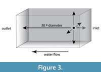
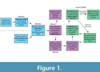A simulation was constructed in three steps; (1) geometry preparation, (2) mesh generation, and (3) numerical model selection (Figure 1). We produced ammonoid shell models in Blender, an open-source, nonspecific 3D geometry creation and manipulation program. We employed a programmer to design Bezier curves to represent aperture shape, set these around a donut-shaped frame, and iterate the size reduction for three whorls until shape parameters (as defined by Westermann, 1996) of the model shell matched those specified by the user to recreate a target specimen or idealized shell geometry. The models explicitly emulate external morphology and present no imitation of internal features relating to either early ontogeny (details of interior whorls at the center of the umbilicus) or void content (internal chamber shape, shell stability, buoyancy, etc.). Models created using Blender were also given no roughness as the shell texture wasn’t a parameter considered in the study. Our models target basic geometry parameters of three different baselines: common morphotypes (Westermann, 1996; Ritterbush and Bottjer, 2012); fossil specimens used in previous physical experiments (Jacobs, 1992); and one laser scan model of a modern Nautilus. The Nautilus model, in contrast to the process described above, was created by smoothing the external surface of single scanned half of the shell and mirroring it to ensure symmetry. These shells and their position in Westermann morphospace are shown in Figure 2. 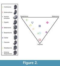Each shell was scaled to 5 cm diameter (measured from the aperture through the central coil; see Smith, 1986) and given a protrusion from the aperture that simulates a simplified soft body extending back approximately 1 cm from the base of the aperture, mimicking previous experiments (Jacobs, 1992). This allows a more direct comparison of the varying shape parameters as variations in overall size, which are known to have a strong effect on hydrodynamics (Klug et al. 2016). Nautilus was used at its full size, 14.5 cm, in addition to version of the same model scaled to 5 cm diameter for comparison with experimental data discussed later.

Each shell was then exported to the modeling program Zbrush for retopology. Retopology is the process of removing internal geometry and recreating the exterior geometry with a uniform distribution of faces at a user-specified resolution (Merlo et al. 2013). Prior to retopology, models are automatically constructed at 1 to 1.5 million face resolutions. These high resolutions allow the software to mathematically meet the specified shape parameters as accurately as possible. However, high resolution models can be computationally expensive and are rarely necessary to preserve the shape following its mathematical construction. Consequently, workstation use benefits from simplification of the shell geometry which, for this study, is achieved by retopology. We chose to simplify the models used in flow studies to a moderate resolution, averaging approximately 30 to 60 thousand faces, which qualitatively preserved the character of the geometry without being computationally expensive.

In mesh generation and numerical simulations, the options available to a user and the performance of simulations will vary with choice of CFD software (Iaccarino, 2001; Glatzel et al., 2008). The present study uses the ANSYS FLUENT V18 as the CFD solver. Other CFD programs exist, including some open source programs, but the ANSYS package was chosen because it offered user-friendly tools and is one of the industry standards (for a more comprehensive discussion of programs see Cunningham et al. 2014). We examined three components that can be varied in constructing a given simulation scheme: the dimensions of the fluid domain, the meshing method used to subdivide the domain, and the turbulence model employed by the solver. These components were varied among four different simulation schemes, which are summarized in Table 1 and are detailed component by component below. These components were varied to achieve results with similar relative accuracy while reducing computational expense. Upon comparison of the results, a scheme that performed in the most accurate and efficient manner was selected and applied to further studies.

FLUENT resolves the flow field of interest using the finite volume method and user specified numerical schemes. Specifically, the user must specify the dimensions of the flow area, and the resolution at which the volume is subdivided for calculation. We used Blender to create a rectangular domain, analogous to the test chamber of a flume or tow tank in physical experiments (such a domain could be created in another program and is down to user preference and comfortability). Domains can either be created to match the dimensions of a test chamber or scaled, based on the model size, to mitigate the effects of flow near walls. Our domains were created with the latter goal in mind, allowing flows to fully develop around the object and minimizing any effects caused by flow near the domain edges. Each domain was scaled relative to the diameter of the shell, aperture to venter (Figure 3). We use a Boolean operation to remove an equivalent space from the domain’s interior mesh. This method makes the domain an expression of the space occupied by the water, rather than an expression of the objects themselves. We examined three different dimension suites for these domains. In schemes 1 and 2, a relatively small domain size was used where the inlet is set at 3 diameters from the object, the outlet is 10 diameters from the object and each wall is 5 diameters from the object. This domain was chosen as a starting point because it has been detailed and successful in previous paleontological studies (Shiino et al., 2009, 2012, 2014). In scheme 3, a larger box was employed to reduce the influence of walls on the flow field development. Here the domain inlet was set 6 diameters from the object, the outlet at 30 diameters, and each wall at 10 diameters. Scheme 4 used a longer box than the other schemes with the outlet at 50 diameters away from the object which allows even more space for the flow field to develop freely. For all of the discussed simulation schemes, we designated the domain’s attributes (inlet, outlet, walls, and ammonoid-shaped obstruction) in the ANSYS DesignModeler module. We employed a uniform velocity inlet (velocity is equal across the whole inlet) with a zero-pressure outlet (no pressure accumulation at the outlet). Finally, all the walls (including the ammonite obstruction) were given a no-slip condition. This method of boundary condition assignment has been verified in previous studies (Day, 1990; Flanagan, 2004; Hannon, 2011; Mossige, 2017). While this is unrealistic for the walls on the outside of the domain, this condition was used to help determine optimal domain sizes. A more realistic setting for the domain walls would be a free slip or symmetry condition where flows near the walls are not treated differently to the regular flow field better representing the open ocean environment.

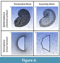
Once the domain of fluid flow is created, the volume is subdivided into a mesh of small 3D cells in a process called volume mesh generation. The solver (ANSYS FLUENT) calculates physical processes (water flow speed and associated forces) over multiple iterations through these cells and finally provides a composite assessment of the computational domain. One key aspect of mesh generation is the geometry of each cell. In Schemes 1 and 4 (Table 1), we employ tetrahedral elements as the base mesh, which is shown to be robust in previous studies for CFD studies and is more appropriate for complex geometry than cube/hex elements (Adkins and Yan, 2006; Rigby and Tabor, 2006; Shiino et al., 2009; Rahman et al., 2015; Dynowski et al. 2016; Rahman, 2017). Scheme 2 applied the ANSYS assembly meshing method, which automatically employs a variety of element types and settings to produce a mesh as a single process. Scheme 3 uses FLUENT’s meshing tools to convert a tetrahedral base mesh into a polyhedral mesh, which decreases total cell count by coupling tetrahedra into unified groups following the initial meshing procedure. Scheme 2, 3, and 4 employ prismatic mesh layers around the edges of the shell-shaped void which, when properly implemented, aid in resolving behavior of the flow near the shell (Shiino et al., 2009, 2012). We chose not to implement this in scheme 1, which we use to assess the method baseline, consistent with previous studies (Rahman et al. 2015).

Fluid flow through the designated space will also depend on its numerical settings and treatment. In FLUENT we defined the fluid as water using the preprogrammed option in all simulations. In all cases, the behavior of these flows are generally governed by the Reynolds-Averaged Navier-Stokes model (Flanagan, 2004; Weymouth et al., 2005; Adkins and Yan, 2006; Rigby and Tabor, 2006; Wilson et al., 2006; Shiino et al., 2009; Hannon, 2011; Dynowski et al. 2016; Mossige, 2017; Rahman, 2017). The standard form of the Navier-Stokes equation mathematically approximates laminar flow and general patterns, but does not account for the complexities that arise from flow instability, such as the occurrence and behavior of turbulent eddies (Argyropoulos and Markatos, 2015; Rahman, 2017). Eddies can be simulated by supplementing the Navier-Stokes equation with additional computational algorithms, the options for which vary by software (Iaccarino, 2001; Argyropoulos and Markatos, 2015). In this study, Scheme 1 uses a realizable k-ε model (Shiino et al., 2009), and the other three schemes employ the Shear Stress Transport (SST) variation of the k-ω model because it combines many of the advantages of the k-ε model, particularly its stability and behavior near boundaries, with those of the more advanced k-ω model, which more accurately resolves smaller scale flow behavior (Argyropoulos and Markatos, 2015).

We ran all simulations in steady state at 11 water velocities ranging from 1 cm/s to 50 cm/s, to address the range of conditions tested in previous studies, but with greater resolution at slower speeds considered more practical for animals of this size (Jacobs 1992). The shell was fixed in a static position in the fluid domain to approximate the animal traveling at a constant speed, mimicking a flume tank experiment. Following comparisons to our baselines, we recorded summary drag force and corresponding coefficient of drag for each water velocity across 11 shell models (Appendix 1 and Appendix 2) using the chosen Scheme. Coefficients of drag were calculated according to Jacobs (1992). Additional investigations of the components of drag (pressure and viscous), as well as overall lift forces, are addressed in forthcoming works of increased scope and specificity.

RESULTS AND DISCUSSION

Evaluation

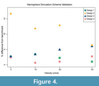We evaluated the performance of each scheme in terms of both its accuracy and computational efficiency. Accuracy was evaluated by comparing the simulated drag force and overall behavior of the simulations to the data of two different benchmarks: analytical solutions for drag on a hemisphere derived from standard coefficient of drag values (Blevins, 1984) and two ammonoid shells used by Jacobs (1992). Any given numerical simulation is, of course, a simplification of the real fluid interactions that the organism would have experienced. Additionally, as described earlier physical experiments have analogous simplifications and noise within their data. For this reason, the objectives of the following numerical comparisons are to replicate the observed trend in the experimental data, and to attain sufficient accuracy that the ranking of the different morphotypes, and the order of magnitude of their drag is preserved. The results of these comparisons are shown in Figure 4 and Figure 5. Efficiency was evaluated based on the total number of mesh elements that result from the simulation scheme employed. The more elements a given system has the more computational resources are required. A scheme that can perform reasonably equally in the accuracy comparisons with fewer overall elements is consequently considered preferable in this study. An average number of elements for each scheme are reported in Table 1.

The accuracy of each method was first evaluated by comparing the simulated drag force to the analytical solution for a hemisphere (Figure 4; raw drag values in Appendix 3); here, both the simulated result and the benchmark are posed in idealized conditions. Most of the simulation schemes provide results in drag force that deviate only a few percent from the benchmarks, with only Scheme 2 showing consistently deviating further from the benchmark solution than the other schemes. The inaccuracy of Scheme 2 likely stems from a combination of the smaller domain introducing wall effects and the assembly meshing method distorting the geometry, an example of which is shown in Figure 6. The other three schemes show a reasonable agreement with the hemisphere benchmark solution. Scheme 4 is the most consistently accurate, but is a much larger mesh, hence higher element count, than the other schemes. Consequently, Scheme 4 has the highest memory requirements of those examined here and substantially longer run times on insufficient hardware. However, the scheme would be optimal if more powerful resources such as high-memory workstation or cluster computing are readily available. Schemes 1 and 3 both perform closely to Scheme 4 with lower computational requirements. Scheme 1’s simulated drag force is more accurate than Scheme 3 at higher velocities as well.

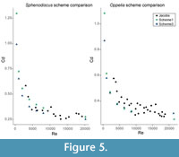
As a second benchmark, Schemes 1 and 3 were compared with the experimental drag coefficient values from Jacobs (1992). For this comparison, data for Sphenodiscus and Oppelia were used as both these shells present smooth surface geometries in Jacobs study, and their morphology could therefore be readily replicated under the same conditions under shells that were constructed. Both schemes follow the trends of these results showing a tight correlation with the clustering of the experimental data (Figure 5). Scheme 3 appears to have a slightly better fit to the Oppelia data, fitting more centrally at higher velocity. Compared to Sphenodiscus the performance of each scheme is comparable with Scheme 1 approximating an upper bound of the data and Scheme 3 approximating a lower bound.

For this study, we prefer the slight underestimation of drag seen in Scheme 3 as it allows us to use our results as maximum swimming efficiencies for each shell, and by consequence their potential end member behaviors. This scheme was also more computationally efficient, with less than half the number of elements in Scheme 1 (Table 1). Additionally, the inclusion of the boundary layer in Scheme 3 provides greater confidence that the flow close to the shell is being accurately resolved (Dynowski et al., 2016). For these reasons we collected the remaining shell data using Scheme 3.

Application

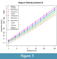Drag forces obtained for all 11 shell models are shown in Figure 7 as a function of velocity. Drag forces are reported in dyne (1e-5 N). Coefficient of drag is also plotted as a function of Reynolds Number in Figure 8. Shells are notably distinct in terms of rank and order of magnitude through the majority of speeds, becoming less distinct at the lower swimming speeds. Two trends emerged when comparing the behavior of drag between across the shell morphologies examined here. First, inflated shells generally produced higher drag than shells of other shapes at comparable diameter and velocity. Second, the range of simulated drag between shapes is highly sensitive to velocity, as highlighted in Figure  7.

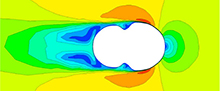
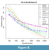The trend of greatest drag variation among ammonoid shells matches expectations from previous work: inflated shell morphologies (i.e., the Nautilus and hypothetical spherocone shells) experience more drag than less-inflated shells (i.e., Sphenodiscus, or the hypothetical Oxycone) (Jacobs, 1992; Westermann, 1996; Ritterbush, 2015). Additionally, inflated shells show a steeper gradient of drag force with changing velocity. This is consistent with the analytical formulation of drag force (D_f =0.5C_d AρU²) where C_d is drag coefficient, A is cross-sectional area, ρ is the density of the fluid, and U is stream velocity. In this formulation, drag force is directly proportional to the square of the stream velocity. When considering this equation using cross-sectional area (A) or volume to the two-thirds power (V^(2/3)), as in Jacobs, 1992), inflated morphologies have a larger cross-sectional area, and consequently the gradient of their drag force is steeper. The second trend, that drag values of these shells become increasingly similar to other morphologies as U, decreases can be explained by the dominant viscous effect in this zone. Inflated shells show consistent and lower change in their coefficient as a function of Reynolds number than the less inflated morphologies (Figure 8). We hypothesize that this may be a result of a behavior shift in how the shell is interacting with the water. At high stream velocities, viscous forces are less likely to play a role in drag because water is being shed from the surface more quickly, leading to small low velocity water zones at the shell surface but large low velocity zone behind the 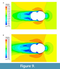shell (Figure 9A). At low stream velocity, these zones are much larger to the sides of the shell but greatly decreased behind it (Figure 9B). This behavior change coincides with a shift of the shell’s characteristic area component from cross-sectional area at high velocities where the shell is being forced through the water to a surface area dominant signal as noted in Jacobs (1992). The surface areas of all these morphologies are much more similar than their cross-sectional areas when their diameter is kept similar, and this could be responsible for the differing gradients. The inflated shells show more consistent drag coefficient values because the change between their cross-sectional area and surface area is much lower than for the less-inflated morphologies. Additional testing will need to be done to test if this behavior is consistent and to potentially characterize the nature of the trade-offs it imposes.

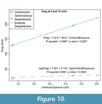In addition to the effect of inflation, the effect of other parameters on drag behavior can be seen, particularly when the inflation of shells is held constant. The degree of umbilical exposure across the central coil appears to substantially influence the widening range of drag between otherwise similar shells with increasing velocity. Figure 10 compares four shell models that have a similar overall thickness ratio - their width at the aperture is 20-22% the value of their diameter - but an order of magnitude difference in the degree of umbilical exposure. The model of Sphenodiscus exposes an umbilical area only 6.2% of the diameter, while the idealized model of an extreme Serpenticone (similar to a sub-adult Dactylioceras) has an umbilical exposure of 60% (see x-axis of Figure 10). Across the examined velocity range, large contrasts in drag correspond to these contrasts in umbilical exposure. At a velocity of 5 cm/s (one shell-diameter per second), umbilical exposure predicts the natural log of the drag, as the contribution of drag over the exposed umbilicus wanes. In contrast, the umbilical exposure creates a profound and linear drag force slope in high stream velocity simulations, shells with stream velocity of 15 cm/s (three shell diameters per second) are shown as an example in Figure 10. We interpret this to be the result of the increased umbilical exposure, in tandem with decreasing whorl expansion, fomenting vortices of water and zones of negative pressure that add resistance against the movement of the 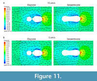shell in the intended direction. These effects can be seen in Figure 11, which shows velocity vectors overlaid on the pressure contours for the surrounding fluid. Shells that express both a greater whorl expansion rate and a covering-over of the umbilical flanks are incredibly common among ammonoids, and the shape trend is named Buckman’s rule (Westermann, 1966; Hammer and Bucher, 2006; Monnet et al., 2015). Our results imply that some hydrodynamic streamlining may follow as an ecological consequence of this shape trend.

Drag force, because it is resistive, must be overcome by an ammonoid in addition to its propulsive requirements to reach a desired speed. This imposes an added energetic cost to swimming, and even subtle changes to such costs may have disproportionate impacts on metabolic demands. Consequently, the nuances highlighted here in both inflation and umbilical exposure might have required alterations in behavior. These nuanced relationships deserve further scrutiny, including hydrodynamics studies focused on the isolation of individual shape variables and how those may favor various swimming behavior.

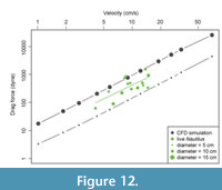Finally, we compared our data for Nautilus pompilius to data collected during a propulsive behavior study (Niel and Askew, 2018; Figure 12). The comparison does not provide sufficient precision to serve as a benchmark by which the CFD methods should be calibrated, but does offer first-order evaluation of the CFD results’ collective accuracy. Our model of Nautilus is based on a single mature specimen and was executed at different sizes in the CFD framework, each with a uniform body extension and a null model of jet behavior by simply moving the water around the model. Niel and Askew (2018) analyzed the volume and velocity of water jets released by live specimens of Nautilus while the animals maneuvered about an experimental water tank. Their published data provide snapshots of apparent drag forces experienced by the animals, but the inherent variability in the experimental design captures a broad variety of conditions: individual animals varied in age and shell size. Isolated jet incidents by each animal additionally varied in body extension, syphon diameter, and jet direction; and total volume and duration of water expulsion. In short, the experimental data are noisy but relevant. Figure 12 shows, in black, the CFD measurements for drag imposed on Nautilus tested at two different sizes, each traveling at the same set of velocities. Data representing apparent drag forces encountered during individual jet events from the experiments by Niel and Askew (2018) are shown in green. The CFD data fit well within the order of magnitude of the drag experienced by live animals, as well as the overall trend in Cd/Re space. This comparison serves two critical purposes. First, it illustrates the potential, and difficulties, of comparing simulation and experimental data. Second, it shows the relevance of CFD methods to resolving trends of physics and ranges of likely behavior that can help design new experiments with both live and model animals.

Considerations for Future Studies

This work presents methods that are convenient and effective for first-order estimates of flow around a nuanced shape. Below, we discuss three approaches that may need to be refined, or given further research, to serve the needs of a wider range of applications.

First, production properties of 3D models should suit their intended purpose or destination. A model intended for CFD simulations may sacrifice external detail (see below) but must satisfy much more strict geometric properties than if it were being printed and physically tested in order to integrate successfully with simulation software. For example, an ammonoid shell model could lack external nuance (i.e., ontogenetic or pathological variation in rib spacing) and still be a useful simulation specimen to test larger morphological trends; but if the same model is rendered incorrectly (i.e., as a series of interlocking but hollow tubes; over smoothing relevant subtle features such concavities into flattened surfaces), it may produce artifacts that overpower or strip out the sought-after signals. Additionally, models created with freestyle tools (e.g., Blender, Maya) or in automated processes (e.g., an adjustable spiral as employed here, or by Raup 1967) commonly employ interior trace intersections, overlapping geometries, or unclean surface mesh models, and these should be made compatible with CFD through retopology. Similarly, models made using photogrammetry, laser scanning, or CT scanning are generally very high fidelity but the surface mesh is typically needlessly dense for CFD applications, particularly if the target variable is a high order variation, such as the broad morphological trends presented here, and can warrant the use of smoothing operations. Such models also tend to produce disorganized, almost random surface meshes with many low-area, inside-out, or otherwise anomalous faces, which can again be rectified through retopology.

In an ideal setting, 3D models used in simulations would provide maximum fidelity relative to their target. In practice, high fidelity simulations are computationally expensive. In many cases, it is advisable to first create a complex model as a baseline, but to then iteratively reduce the complexity to suit each task. A model produced from a laser or CT scan might have millions of geometric faces, but an iterated decimation operation (reducing the face count by an order of magnitude each time) can yield a model better-suited for morphometric or CFD analysis (e.g., Adkins and Yan, 2006; Bates et al., 2009; Rahman et al., 2015; Liu et al., 2015). Custom reduction in model complexity can be time-consuming or expensive, however, so high-complexity models are not always a necessary starting point. Studies of structure (reaction to stress, pressure, or bite forces) will be sensitive to model complexity in different ways than CFD, and relevant model considerations are presented in simulations that use Finite Elements Analysis (e.g., Dumont et al., 2009; Snively and Theodor, 2011; Lautenschlager, 2013; Lemanis et al., 2016). The main benefit of 3D models produced under these considerations means that they can be shared among researchers and used without need for significant alteration, affording a level of reproducibility that is difficult to achieve with physical experiments and models.

Finally, turbulence models can greatly influence CFD simulations and must be chosen carefully. Ultimately, numerical models are only an approximation of the physical world. When modeling ancient and extinct organisms, validation of numerical models to physical experiments are not always possible. In such cases, it is necessary to apply different numerical schemes and do sensitivity analyses to gain confidence in the numerical results, with the exact choices made varying between organisms. CFD methods are simplifications with well-known philosophical caveats (Spalart, 2015), and researchers may choose the set of assumptions that most emphasize the phenomena under investigation. In this study, the complexity of ammonoid shell spirals was well suited for use with the SST k-ω model, which can allow greater variation within particular elements of the fluid space. Models with k-ε variations are prone to more uniform treatment of the mathematics throughout a problem (Argyropoulos and Markatos, 2015), and may provide greater consistency when repeated. It is also important to acknowledge that Reynolds-averaged simulation methods like these, despite being commonly employed, are also mere approximations of real-world complexity. For ammonoid hydrodynamics, as for all paleontological uses, future interpretations will be well served by continued attention to advances in CFD tools and their increasing application (turbulence tuning, grid-less methods, etc.).

CONCLUSION

Applying modern 3D-CFD simulations methods shows considerable promise for advancing paleobiological research. In this study we use these tools to produce a range of ammonoid shell morphologies, both idealized morphotypes and fossil reconstructions. By employing the developed 3D geometries in CFD simulations, we were able to show that an ammonoid's swimming capability is strongly influenced by overt parameters such as width. We also found that even subtle differences in coiling between otherwise similarly proportioned morphologies result in noticeable changes in bioenergetic requirements. Subtle changes such as these have the potential to dramatically impact interpretations of the role ammonoids play in paleoecosystems and how marine trophic systems may evolve through deep time (Tajika, et al. 2018; Walton and Korn, 2018).

Future work employing these tools has the potential to be some of the most impactful, reproducible, and distributable yet. This unprecedented communicability also means that researchers must focus even more on reporting the protocols used for creating models and simulations. Doing so will help to maintain relevant and well-developed data sets and facilitate additional improvements upon protocols like the simple guidelines we present in this paper.

ACKNOWLEDGEMENTS

We would like the thank C. Haug and two anonymous reviewers whose comments and suggestions helped tremendously improve and clarify the core of this paper. We would also like to thank R. Irmis, S. Naleway, J. Moore, M. Clapham, and T. Faith for their support and input as this paper was being prepared.

REFERENCES

Adkins, D. and Yan, Y. 2006. CFD simulation of fish-like body moving in viscous liquid. Journal of Bionic Engineering, 3:147-153. https://doi.org/10.1016/S1672-6529(06)60018-8

Argyropoulos, C.D. and Markatos, N.C. 2015. Recent advances on the numerical modelling of turbulent flows. Applied Mathematical Modelling, 39:693-732. https://doi.org/10.1016/j.apm.2014.07.001

Batt, R.J. 1989. Ammonite shell morphotype distributions in the western interior Greenhorn Sea and some paleoecological implications. Palaios, 4:32-42. https://doi.org/10.2307/3514731

Blevins, R.D. 1984. Applied Fluid Dynamics Handbook. Van Nostrand Reinhold Co., New York City, New York.

Chamberlain, J.A. 1976. Flow patterns and drag coefficients of cephalopod shells. Palaeontology, 19:539-563.

Chamberlain, J.A. 1980. The role of body extension in cephalopod locomotion. Palaeontology, 23:445-461.

Chamberlain, J.A. and Westermann, G.E.G. 1976. Hydrodynamic properties of cephalopod shell ornament. Paleobiology, 2:316-331.

Cunningham, J.A., Rahman, I.A., Lautenschlager, S., Rayfield, E.J., and Donoghue, P.C.J. 2014. A virtual world of paleontology. Trends in Ecology & Evolution, 29:347-357. https://doi.org/10.1016/j.tree.2014.04.004

Day, M.A. 1990. The no-slip condition of fluid dynamics. Erkenntnis, 33:285-296.

Dumont, E.R., Grosse, I.R., and Slater, G.J. 2009. Requirements for comparing the performance of finite element models of biological structures. Journal of Theoretical Biology, 256:96-103. https://doi.org/10.1016/j.jtbi.2008.08.017

Dynowski, J.F., Nebelsick, J.H., Klein, A., and Roth-Nebelsick, A. 2016. Computational fluid dynamics analysis of the fossil crinoid Encrinus liliiformis (Echinodermata: Crinoidea). PLOS ONE, 11:e0156408. https://doi.org/10.1371/journal.pone.0156408

Flanagan, P.J. 2004. Unsteady Navier-Stokes Simulation of Rainbow Trout Swimming Hydrodynamics. Unpublished Master’s Thesis, Washington State University, Pullman, Washington, USA.

Glatzel, T., Litterst, C., Cupelli, C., Lindemann, T., Moosmann, C., Niekrawietz, R., Streule, W., Zengerle, R., and Koltay, P. 2008. Computational fluid dynamics (CFD) software tools for microfluidic applications - A case study. Computers & Fluids, 37:218-235. https://doi.org/10.1016/j.compfluid.2007.07.014

Hammer, O. and Bucher, H. 2006. Generalized ammonoid hydrostatics modelling, with application to Intornites and intraspecific variation in Amaltheus. Paleontological Research, 10:91-96. https://doi.org/10.2517/prpsj.10.91

Hannon, J.W. 2011. Image Based Computational Fluid Dynamics Modeling to Simulate Fluid Flow around a Moving Fish. Unpublished Master’s Thesis, The University of Iowa, Iowa City, Iowa, USA.

Iaccarino, G. 2001. Predictions of a turbulent separated flow using commercial CFD codes. Journal of Fluids Engineering, 123:819-828. https://doi.org/10.1115/1.1400749

Jacobs, D.K. 1992. Shape, drag, and power in ammonoid swimming. Paleobiology, 18:203-220. https://doi.org/10.1017/S009483730001397X

Jacobs, D.K. and Landman, N.H. 1993. Nautilus—a poor model for the function and behavior of ammonoids? Lethaia, 26:101-111. https://doi.org/10.1111/j.1502-3931.1993.tb01799.x

Klug, C., De Baets, K., and Korn, D. 2016. Exploring the limits of morphospace: ontogeny and ecology of late Viséan ammonoids from the Tafilalt, Morocco. Acta Palaeontologica Polonica, 61(1):1-14. https://doi.org/10.4202/app.00220.2015

Klug C., Korn D., De Baets K., Kruta I., Mapes R. 2015a. Ammonoid Paleobiology: From Macroevolution to Paleogeography. Topics in Geobiology, 44. Springer, Dordrecht, Netherlands. https://doi.org/10.1007/978-94-017-9633-0

Klug C., Kröger B., Vinther J., Fuchs D., De Baets K. 2015b. Ancestry, origin and early evolution of ammonoids. p. 3-24. In: Klug C., Korn D., De Baets K., Kruta I., and Mapes R. (eds.), Ammonoid Paleobiology: From Macroevolution to Paleogeography. Topics in Geobiology, vol 44. Springer, Dordrecht, Netherlands. https://doi.org/10.1007/978-94-017-9633-0_1

Kröger, B., Vinther, J., and Fuchs, D. 2011. Cephalopod origin and evolution: A congruent picture emerging from fossils, development and molecules. BioEssays, 33:602-613. https://doi.org/10.1002/bies.201100001

Lautenschlager, S. 2013. Cranial myology and bite force performance of Erlikosaurus andrewsi: a novel approach for digital muscle reconstructions. Journal of Anatomy, 222:260-272. https://doi.org/10.1111/joa.12000

Lemanis, R., Zachow, S., and Hoffmann, R. 2016. Comparative cephalopod shell strength and the role of septum morphology on stress distribution. PeerJ, 4:e2434. https://doi.org/10.7717/peerj.2434

Liu, S., Smith, A.S., Gu, Y., Tan, J., Liu, C.K., and Turk, G. 2015. Computer simulations imply forelimb-dominated underwater flight in plesiosaurs. PLOS Computational Biology, 11:e1004605. https://doi.org/10.1371/journal.pcbi.1004605

Merlo, A., Sánchez Belenguer, C., Vendrell Vidal, E., Fantini, F., and Aliperta, A. 2013. 3D model and visualization enhancements in real-time game engines. ISPRS - International Archives of the Photogrammetry, Remote Sensing and Spatial Information Sciences, XL-5/W1:181-188. https://doi.org/10.5194/isprsarchives-XL-5-W1-181-2013

Monnet, C., De Baets, K., and Yacobucci, M.M. 2015. Buckman’s rules of covariation, p. 67-94. In Klug C., Korn D., De Baets K., Kruta I., and Mapes, R. (eds.), Ammonoid Paleobiology: From Macroevolution to Paleogeography. Topics in Geobiology, 44. Springer, Dordrecht, Netherlands. https://doi.org/10.1007/978-94-017-9633-0_4

Mossige, J.C. 2017. Numerical Simulations of Swimming Fish. Unpublished Master’s Thesis, Norwegian University of Science and Technology, Trondheim, Norway.

Naglik C., Tajika A., Chamberlain J., Klug C. 2015. Ammonoid locomotion. In: Klug C., Korn D., De Baets K., Kruta I., and Mapes R. (eds.), Ammonoid Paleobiology: From Anatomy to Ecology. Topics in Geobiology, 43. Springer, Dordrecht, Netherlands. https://doi.org/10.1007/978-94-017-9630-9_17

Neil, T.R. and Askew, G.N. 2018. Swimming mechanics and propulsive efficiency in the chambered nautilus. Royal Society Open Science, 5:170467. https://doi.org/10.1098/rsos.170467

Rahman, I.A. 2017. Computational fluid dynamics as a tool for testing functional and ecological hypotheses in fossil taxa. Palaeontology, 60:451-459. https://doi.org/10.1111/pala.12295

Rahman, I.A., Zamora, S., Falkingham, P.L., and Phillips, J.C. 2015. Cambrian cinctan echinoderms shed light on feeding in the ancestral deuterostome. Proceedings of the Royal Society B: Biological Sciences, 282:20151964. https://doi.org/10.1098/rspb.2015.1964

Raup, D.M. 1967. Geometric analysis of shell coiling: coiling in ammonoids. Journal of Paleontology, 41:43-65.

Rigby, S. and Tabor, G. 2006. The use of computational fluid dynamics in reconstructing the hydrodynamic properties of graptolites. GFF, 128:189-194. https://doi.org/10.1080/11035890601282189

Ritterbush, K.A. 2015. Interpreting drag consequences of ammonoid shells by comparing studies in Westermann Morphospace. Swiss Journal of Palaeontology, 135:125-138. https://doi.org/10.1007/s13358-015-0096-8

Ritterbush, K.A. and Bottjer, D.J. 2012. Westermann Morphospace displays ammonoid shell shape and hypothetical paleoecology. Paleobiology, 38:424-446. https://doi.org/10.1666/10027.1

Ritterbush, K.A. and Foote, M. 2017. Association between geographic range and initial survival of Mesozoic marine animal genera: circumventing the confounding effects of temporal and taxonomic heterogeneity. Paleobiology, 43:209-223. https://doi.org/10.1017/pab.2016.25

Ritterbush, K.A., Hoffmann, R., Lukeneder, A., and De Baets, K. 2014. Pelagic palaeoecology: the importance of recent constraints on ammonoid palaeobiology and life history: pelagic palaeoecology of ammonoids. Journal of Zoology, 292:229-241. https://doi.org/10.1111/jzo.12118

Shiino, Y., Kuwazuru, O., Suzuki, Y., and Ono, S. 2012. Swimming capability of the remopleuridid trilobite Hypodicranotus striatus: Hydrodynamic functions of the exoskeleton and the long, forked hypostome. Journal of Theoretical Biology, 300:29-38. https://doi.org/10.1016/j.jtbi.2012.01.012

Shiino, Y., Kuwazuru, O., Suzuki, Y., Ono, S., and Masuda, C. 2014. Pelagic or benthic? Mode of life of the remopleuridid trilobite Hypodicranotus striatulus. Bulletin of Geosciences, 89:207-218. https://doi.org/10.3140/bull.geosci.1409

Shiino, Y., Kuwazuru, O., and Yoshikawa, N. 2009. Computational fluid dynamics simulations on a Devonian spiriferid Paraspirifer bownockeri (Brachiopoda): Generating mechanism of passive feeding flows. Journal of Theoretical Biology, 259:132-141. https://doi.org/10.1016/j.jtbi.2009.02.018

Smith, P.L. 1986. The implications of data base management systems to paleontology: a discussion of Jurassic ammonoid data. Journal of Paleontology, 60:327-340. https://doi.org/10.1017/S0022336000021843

Smith, P.L., Longridge, L.M., Grey, M., Zhang, J., and Liang, B. 2014. From near extinction to recovery: Late Triassic to Middle Jurassic ammonoid shell geometry. Lethaia, 47:337-351. https://doi.org/10.1111/let.12058

Snively, E. and Theodor, J.M. 2011. Common functional correlates of head-strike behavior in the pachycephalosaur Stegoceras validum (Ornithischia, Dinosauria) and combative artiodactyls. PLoS ONE, 6:e21422. https://doi.org/10.1371/journal.pone.0021422

Spalart, P.R. 2015. Philosophies and fallacies in turbulence modeling. Progress in Aerospace Sciences, 74:1-15. https://doi.org/10.1016/j.paerosci.2014.12.004

Tajika, A., Nützel, A., and Klug, C. 2018. The old and the new plankton: ecological replacement of associations of mollusc plankton and giant filter feeders after the Cretaceous? PeerJ, 6:e4219. https://doi.org/10.7717/peerj.4219

Tendler, A., Mayo, A., and Alon, U. 2015. Evolutionary tradeoffs, Pareto optimality and the morphology of ammonite shells. BMC Systems Biology, 9(12):1-12. https://doi.org/10.1186/s12918-015-0149-z

Walton, S.A. and Korn, D. 2018. An ecomorphospace for the Ammonoidea. Paleobiology, 44:273-289. https://doi.org/10.1017/pab.2017.33

Ward, P. 1980. Comparative shell shape distributions in Jurassic-Cretaceous ammonites and Jurassic-Tertiary nautilids. Paleobiology, 6:32-43. https://doi.org/10.1017/S0094837300012471

Westermann, G. 1966. Covariation and taxonomy of the Jurassic ammonite Sonninia adicra (Waagen). Neues Jahrbuch fur Geologie und Palaontologie, Abhandlungen, 124:289-312.

Westermann G.E.G. 1996. Ammonoid life and habitat, p. 607-707. In Landman N.H., Tanabe K., and Davis R.A. (eds.), Ammonoid Paleobiology. Topics in Geobiology, 13. Springer, Boston, Massachusetts. https://doi.org/10.1007/978-1-4757-9153-2_16

Wilson, R.V., Carrica, P.M., and Stern, F. 2006. Unsteady RANS method for ship motions with application to roll for a surface combatant. Computers & Fluids, 35:501-524. https://doi.org/10.1016/j.compfluid.2004.12.005